88쪽
원시 변수는 변수의 실제 값을 나타내는 비트가 들어있지만,
객체 레퍼런스에는 객체에 접근하는 방법을 알려주는 비트가 들어있다. (비트 수는 중요하지 않다.)
(객체 자체는 변수에 저장되지 않는다.)
(96쪽) 레퍼런스 변수의 값은 힙에 들어있는 객체를 건드릴 수 있는 방법을 나타내는 비트. 레퍼런스 변수가 아무 객체도 참조하지 않으면 그 값은 null이 됩니다.
89쪽 객체 선언/생성/대입의 3단계 1. 레퍼런스 변수 선언 (객체를 제어하기 위한 레퍼런스 변수용 공간을 할당) 2. 객체 생성 (힙에 새로운 객체를 위한 공간을 마련) 3. 객체와 레퍼런스 연결 (새로운 객체를 레퍼런스 변수에 대입)
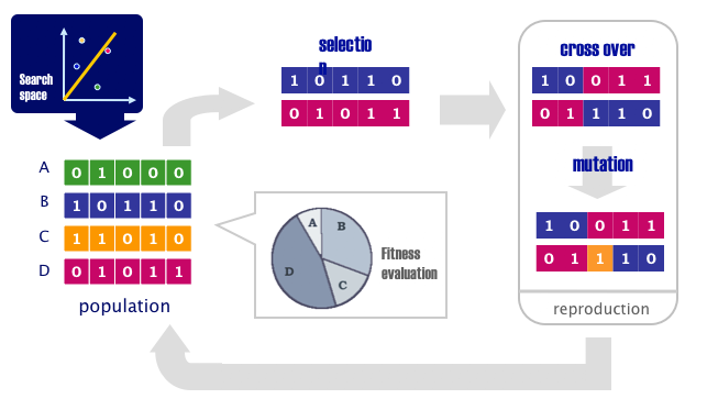
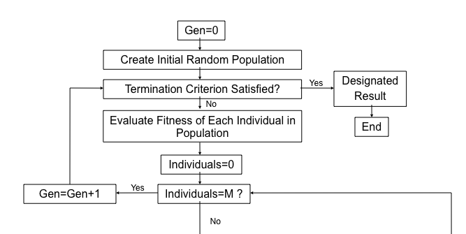
함수 리스트에서 {+, *, cos, ..., minus} random하게 선택하여 (uniform distribution) Tree의 root로 삼는다. depth 만큼 Tree를 생성하고 나면, 단말 리스트에서 random하게 선택하여 Tree의 leaf로 삼는다
주어진 depth에 대해 (1) 상수일지 함수일지 선택 (2) 상수이면 leaf가 되는 것이고, 함수이면 다음 depth를 생성한다.
if (current.depth < maximum.depth) { 함수 선택 }
1. Class Tree를 만들고 2. Tree instance를 여러 개 만들어서 list로 만든다. 3. 주어진 depth에 대해 2로부터 random choice로 Tree 구조를 생성한다. "Left를 먼저 채울지 Right를 먼저 채울지도 random으로 선택"
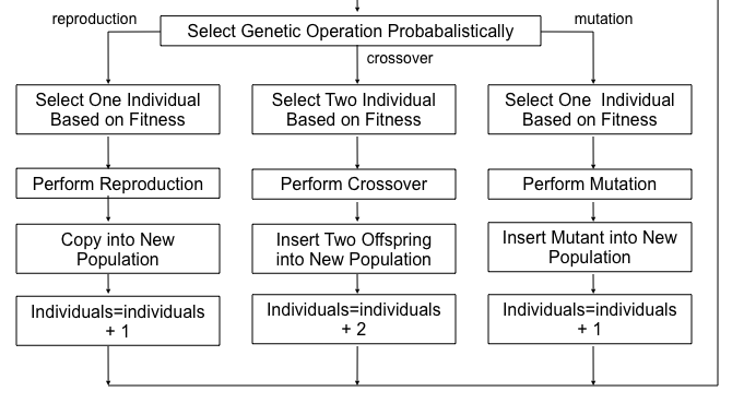
2) mutation과 combination
방법 1. mutation이 일어날 Tree를 random하게 (낮은 비율로) 선택한다. 2. 각 node를 방문하여 mutation의 여부를 결정한다. 3.
Data Type 1) boolean 2) byte 3) char 4) int 5) float 6) color
* float이 memory를 훨씬 많이 차지하므로 정수는 int로 선언한다. float f; f = 2.7; int i = (int) f; //i=2가 된다.
똑같은 성질을 가지는 변수들이 여러 개일 때 array를 쓴다. 1024*768 (1280*1024)
변수명 붙이는 요령: 1. meaning 2. 소문자+대문자 (eg. roomTemp)
1) element: VarX (10%), VarY(30%), A(40%), B(20%) 2) array를 만든다 (길이 10) {VarX, VarY, VarY, VarY, A, A, A, A, B, B} a) random number를 선택한다 rnum = random(0, 1) (-> 항상 float) rnum = random(0, 10) (int) rnum b) if (0~4) {VarX}
(각 op가 뽑힐 확률은 지정해 둔다.) selection을 (충분히 많이) 무한 번 반복하면 각 op가 가지는 확률을 알 수 있다.
tree 1과 tree 2를 교배시켜 새로운 tree 3을 생성할 때, 각 tree 1과 tree 2의 요소(node)가 변이(mutation)을 일으킬 수 있다.
mutation
tree의 각 node에서 mutation이 일어날 확률을(여부를) 계산(선택)한다. 즉, 각 node마다 mutation probability를 가진다. (그림)
cross-over
(그림)
(1/2)*(1/2) = 1/4 그러나 (유전자 쌍의 동일한 위치에서 일어나는) cross-over 때문에 매번 다른 유전자를 지닌 자식이 나온다. => "phenotype" 대응되는 node끼리 교배 -> 우열 등의 규칙은 임의로 결정
(그림)
tree 하나를 염색체 하나로 보고 유전 법칙을 적용하자. 염색체가 (이중나선 DNA)쌍으로 존재하듯, 염색체 한 쌍을 보유하는 개체 하나 당 tree 2개로 구성되어 있다고 본다. 교배는 이 개체와 다른 개체, 즉 총 4개의 tree가 mutation, cross-over 수반한 교배를 한다. 이렇게 생성된 evolved 이미지에 criteria를 적용하여 적자생존의 법칙처럼 적당한 이미지가 걸러지도록 한다.
ref. Steve Oualline, Practical C Programmin, 292-293p
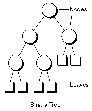
root node leaves
"Recursion is extremely useful with trees. Our rules for recursion are: 1. The function must make things simpler. This rule is satisfied by trees, because as you descend the hierarchy there is less to search. 2. There must be some endpoint. A tree offers two endpoints, either you find a match, or you reach a null node.
Non-Uniform Random Variate Generation (originally published with Springer-Verlag, New York, 1986) Luc Devroye School of Computer Science McGill University
III. DISCRETE RANDOM VARIATES 83 1. Introduction. 83 2. The inversion method. 85 2.1. Introduction. 85 2.2. Inversion by truncation of a continuous random variate. 87
The word entheogen is derived from the ancient Greek : ἔνθεος (entheos) and γενέσθαι (genesthe). Entheos
literally means "god (theos) within", translates as "inspired" and is
the root of the English word "enthusiasm". The Greeks used it as a term
of praise for poets and other artists. Genesthe
means "to generate". So an entheogen is "that which generates God (or
godly inspiration) within a person". (중략) It was coined as a
replacement for the terms "hallucinogen" (popularized by Aldous Huxley's experiences with mescaline, published as The Doors of Perception in 1953) and "psychedelic" (a Greek neologism for "mind manifest", coined by psychiatrist Humphry Osmond,
who was quite surprised when the well-known author, Aldous Huxley,
volunteered to be a subject in experiments Osmond was running on
mescaline). Ruck et al. argued that the term "hallucinogen" was
inappropriate due to its etymological relationship to words relating to
delirium and insanity. The term "psychedelic" was also seen as problematic, due to the similarity in sound to words pertaining to psychosis and also due to the fact that it had become irreversibly associated with various connotations of 1960spop culture.
(아~ 또 삼천포. 그만 가야지...)
keywords: random, Brownian motion, Tydall effect, random walk, mean square distance, Monte Carlo (여기에도 나오네... 적분 방법 아니었어?), pseudo-random number generators (그래 이게 목적이겠지만.), Molecular Dynamics (MD) 방법 (방법??), self-avoiding random walk (SAW), Flory 이론, Nienhuis (??), persistent random walk, limited random walk, fractal growth, DLA (Diffusion Limited Aggregates), Chaos Game, Iterated Function System, Theory of Affine Map (->Image Processing), Benoit Mandelbrot, Fractal Geometry, Hausdorff Dimension, Koch 곡선, Box counting algorithm (Capacity dimension), 'Mountains Never Existed',
MC(Monte Carlo) code:
if randN(m) < 0.5,
Point(m) = Point(m)+1;
else
Point(m) = Point(m)-1;
end;
randN = rand(N) : Generate N random number between 0 and 1
MC 방법의 응용 * random walks, fractal growth, * Equilibrium/non-equilibrium statistical phenomena, phase transition * neural networks * particle scattering with the help of computers * optimization 나는 particle scattering 때문에 자주 본 거였구만.
RAND(N) (0.0,1.0)사이의 균일한 분포를 가진 마구잡이 수로 이루어진 NxN 행렬 그럼 프로세싱에서의 random()인 건가...? 분포가 다른 건가?
S = RAND('state') 현재상태를 포함한 35-element 벡터. RAND('state',S) resets the state to S. RAND('state',0) resets the generator to its initial state. RAND('state',J), for integer J, resets the generator to its J-th state. RAND('state',sum(100*clock)) resets it to a different state each time. 포기.
ref. K. Kremer and T. W. Lyklema, Phys. Rev. Lett. 55, 9091 (1985) T. M. Bishtein, S. V. Buldyrev, and A. M. Elyashivitch, Polymer 26, 1814 (1985)
Fractal Growth
- 평형으로부터 멀리 떨어진 현상 (far from equilibrium)
- 시공간적으로 매우 다양한 형태
- 해석적 연구가 매우 어려움
프랙탈 성장의 예
- 금속이온의 전기화학적 흡착에 의한 뭉침
- 고분자, 세라믹, 유리, 얇은막의 성장
- Viscous fingering
- Dielectric breakdown
- 박테리아의 성장
- 신경세포의 성장
* 성장규칙 o 평면상의 움직이지 않는 씨앗으로부터 시작. o 멀리 떨어진 곳으로부터 시작하여 마구 걷기를 수행. o 마구 걷기가 씨앗을 만나면 붙음. o 다시 마구걷기를 반복함._M#]
Mountains Never Existed
Iterated Function System
The concept of the Iterated Function System was invented by creative fractal genius Michael Barnsley. An IFS is composed of a few simple elements: transformations and probabilities. The transformations are usually expressed as matrices--one translational matrix and one transformational matrix. This sounds a bit dry, but actually the concept is a bit more interesting than all that. For the Sierpinski Triangle, the transformations are simple, and are better expressed as rules in a recursive procedure:
Begin by selecting three vertices in the two-dimensional plane. Note their coordinates. Next, select an initial point--best if within the bounds of the triangle formed by the three vertices, but this is not a requirement. The main procedure goes as follows.
Select one of the three vertices at random.
Roll a six sided die and integer-divide by two, flip three coins and take the exception, or ask a friendly computer for help.
From the current location of the point, calculate the midpoint of the line connecting the point and the vertex just selected.
Move to this midpoint, and plot the point.
Iterate ad infinitum.
That's it! Sierpinski's Triangle. To get any sort of worthwhile picture, of course, hundreds to thousands of points need to be plotted. In fact, usually the first twenty or so points are off track and need not be plotted. However, the algorithm outlined above is amazingly simple to do, and incredibly easy to implement on any machine. I have written Sierpinski programs for every graphing calculator under the sun, as well as for most desktop computers as well. Try
it yourself in BASIC or on a graphing calculator. You'll surprise yourself at how easy it is to impress people with a graphing calculator. :)
How Long is the Coast?
A long, long time ago, fractal god Benoit Mandelbrot posed a whimsical question: How long is the coastline of Britain? His mathematical colleagues were miffed, to say the least, at such annoying waste of their amazing computation powers on this insignificant minutae. They told him to look it up.
Of course, Mandelbrot had a reason for his peculiar question. Quite an interesting reason. Look up the coastline of Britain yourself, in some encyclopedia. Whatever figure you get, it is wrong. Quite simply, the coastline of Britain is infinite. You protest that this is impossible. Well, consider this. Consider looking at Britain on a very large-scale map. Draw the simplest two-dimensional shape possible, a triangle, which circumscribes Britain as closely as possible. The perimeter of this shape approximates the perimeter of Britain.However, this area is of course highly inaccurate. Increasing the amount of vertices of the shape going around the coastline, and the area will become closer. The more vertices there are, the closer the circumscribing line will be able to conform to the dips and the protrusions of Britain's rugged coast.There is one problem, however. Each time the number of vertices increases, the perimeter increases. It must increase, because of the triangle inequality. Moreover, the number of vertices never reaches a
maximum. There is no point at which one can say that a shape defines the coastline of Britain. After all, exactly circumscribing the coast of Britain would entail encircling every rock, every tide pool, every pebble which happens to lie on the edge of Britain. Thus, the coastline of Britain is infinite.
The dependence of length (or area) measurements on scale poses great problems for biologists who need to use the results. For example, lakes that have a very convoluted shoreline are known to offer more area of shallows in relation to their total surface area, and thus support richer communities of plant and animal life. Attempts to characterize shore-line communities in terms of indexes that relate water surface to shoreline length have been frustrated by problems of scale.
Fractal dimension
The notion of "fractional dimension" provides a way to measure how rough fractal curves are. We normally consider lines to have a dimension of 1, surfaces a dimension of 2 and solids a dimension of 3. However, a rough curve (say) wanders around on a surface; in the extreme it may be so rough that it effectively fills the surface on which it lies. Very convoluted surfaces, such as a tree's foliage or the internal surfaces of lungs, may effectively be three-dimensional structures. We can therefore think of roughness as an increase in dimension: a rough curve has adimension between 1 and 2, and a rough surface has a dimension somewhere between 2 and 3. The dimension of a fractal curve is a number that characterizes the way in which the measured length between given points increases as scale decreases. Whilst the topological dimension of a line is always 1 and that of a surface always 2, the fractal dimension may be any real number between 1 and 2. The fractal dimension D is defined by
log ( L2 / L1 )
D = --------------- ... (1)
log ( S1 / S2 )
where L1, L2 are the measured lengths of the curves (in units), and S1, S2 are the sizes of the units (i.e. the scales) used in the measurements.
Van Koch Curve
This is the Von Koch curve. Its construction is almost as easy as the Sierpinski Triangle. You start with a triangle (equilaterality is really more important in this case than for the Sierpinski Triangle), and, on each side, tack on little equilateral triangles, so you end up with a shape very much like a Star of David. The Star of David has six little triangles sticking out. For each triangle, repeat the previous process. Iterate infinitely.
Recall that when we discussed the Koch Curve in figure 4(b), we had four chunks that were small copies of the whole curve. Each chunk could be magnified by 3 to return a copy the same size as the original curve. Plugging these values into the above equation, we get
Ds = log4 /log3= 1.262
This is a value we would have expected. Because the curve is more intricate than a 1-dimensional line segment (it wanders around on the plane some), we would expect its fractal dimension to be greater than 1. But it doesn't come very close to filling an area of the 2-dimensional plane, so we would expect the curve's fractal dimension to be much smaller than 2. The Koch Curve is indeed a fractal. It is self-similar and it has a fractional dimension of about 1.262.
Sierpinsky Gasket
Now the Sierpinski Gasket of figure 2 comes a little closer to filling a 2-dimensional triangle, so we will expect it to have a fractal dimension closer to 2. Recall that we have 3 subtriangles that can be magnified by 2 to get back a copy the same size as the original. Plugging those values into the Self-Similarity dimension equation, we get
Ds = log3/log2= 1.585
The Sierpinski Gasket is therefore a fractal--It is self-similar and its fractional dimension is about 1.585. We have now investigated two bonafide fractals. Both the Sierpinski Gasket and the Koch Curve satisfy Devaney's two criteria for being a fractal: self-similarity and fractional dimension.
Reductionism is the idea that a system can be understood by examining its individual parts. (Implicit in this idea is that one may have to examine something at multiple levels.)
Traditional scientists study two types of phenomena: agents and interactions of agents.
1) 환원주의적 접근으로 해부하기 2) 보다 넓은 시야로 전체 집합을 이해하기 - 몇 개의 agents가 전체적인 패턴을 형성하는지 (예) 뇌세포:인간 지능) 3) 1과 2의 사이에서 agents 간의 상호작용을 연구하기 - The interactions of agents can be seen to form the glue that binds one level of understanding to the next level.
1.1 Simplicity and Complexity
emergent의 예: 개미 굴/군집, 예측을 벗어나는 경제 시장, 척추동물의 패턴 인식 능력, 바이러스와 박테리아에 저항하는 인간의 면역 체계, 지구 생명체의 진화 => 간단한 단위들로 이루어져 있는데 결합하면 전체적으로 복잡한 형상을 띤다. => 단지 부분들의 합으로는 설명할 수 없는 거대한 체계를 이룬다.
The whole of the system is greater than the sum of the parts(, which is a fair definition of holism -- the very opposite of reductionism).
Agents that exist on one level of understanding are very different from agents on another level. Yet the interactions on one level of understanding are often very similar to the interactions on other levels.
상사12 (相似) 「명」「1」서로 모양이 비슷함. 「2」『생』종류가 다른 생물의 기관이 발생적으로 기원과 구조가 다르나 형상과 작용이 서로 일치하는 현상. 예를 들면, 새의 날개와 벌레의 날개 관계, 또는 잎이 변하여 된 완두콩의 덩굴손과 줄기가 변하여 된 포도 나무의 덩굴손 관계 따위이다. 「3」『수1』=닮음〔1〕. 「참」상동04(相同).
ref. 표준국어대사전
# 예측불능성 (unpredictability) 예) 주식 시장, 날씨
# 복잡성 complexity 예) 개미 군, 인간 뇌, 경제 시장 => By self-organizing, complex behavior of collectives is much richer than the behavior of the individual component units.

 invalid-file