OpenCV 함수 cvFindChessboardCorners()와 cvDrawChessboardCorners() 사용
-
bool findChessboardCorners(const Mat& image, Size patternSize, vector<Point2f>& corners, int flags=CV_CALIB_CB_ADAPTIVE_THRESH+ CV_CALIB_CB_NORMALIZE_IMAGE)
Finds the positions of the internal corners of the chessboard.
file:///Users/lym/opencv/src/cv/cvcalibinit.cpp
https://code.ros.org/trac/opencv/browser/tags/2.1/opencv/src/cv/cvcalibinit.cpp
void drawChessboardCorners(Mat&
image, Size
patternSize, const
Mat&
corners, bool
patternWasFound)Renders the detected chessboard corners.
| Parameters: |
- image – The destination image; it must be an 8-bit color image
- patternSize – The number of inner corners per chessboard
row and column. (patternSize = cvSize(points _ per _ row,points _ per _
colum) = cvSize(columns,rows) )
- corners – The array of corners detected
- patternWasFound – Indicates whether the complete board was found or not . One may just pass the return value FindChessboardCorners her
|
Learning OpenCV: Chapter 11. Camera Models and Calibration: Chessboards
381p

640x480
console:
finding chessboard corners...
what = 1
chessboard corners: 215.5, 179
#0=(215.5, 179) #1=(237.5, 178.5) #2=(260.5, 178) #3=(283.5, 177.5) #4=(307, 177) #5=(331.5, 175.5) #6=(355.5, 174.5) #7=(380.5, 174) #8=(405.5, 173.5) #9=(430.5, 172.5) #10=(212.5, 201.5) #11=(235.5, 201.5) #12=(258, 200.5) #13=(280.5, 200.5) #14=(305.5, 199.5) #15=(330, 198.5) #16=(354.5, 198) #17=(379.5, 197.5) #18=(405.5, 196.5) #19=(430.5, 196) #20=(210, 224.5) #21=(232.5, 224.5) #22=(256, 223.5) #23=(280, 224) #24=(304, 223) #25=(328.5, 222.5) #26=(353.5, 222) #27=(378.5, 221.5) #28=(404.5, 221.5) #29=(430.5, 220.5) #30=(207, 247.5) #31=(230.5, 247.5) #32=(253.5, 247.5) #33=(277.5, 247) #34=(303, 247) #35=(327, 246.5) #36=(352, 246.5) #37=(377.5, 246) #38=(403.5, 245.5) #39=(430, 245.5) #40=(204.5, 271.5) #41=(227.5, 271.5) #42=(251.5, 271.5) #43=(275.5, 271.5) #44=(300, 272) #45=(325.5, 271.5) #46=(351, 271) #47=(376.5, 271.5) #48=(403, 271.5) #49=(429.5, 271) #50=(201.5, 295.5) #51=(225.5, 295.5) #52=(249.5, 296) #53=(273.5, 296.5) #54=(299, 297) #55=(324, 296) #56=(349.5, 296.5) #57=(375.5, 296.5) #58=(402.5, 296.5) #59=(429, 297)
finished

finding chessboard corners...
what = 0
chessboard corners: 0, 0
#0=(0, 0) #1=(0, 0) #2=(0, 0) #3=(0, 0) #4=(0, 0) #5=(0, 0) #6=(0, 0) #7=(0, 0) #8=(0, 0) #9=(0, 0) #10=(0, 0) #11=(0, 0) #12=(0, 0) #13=(0, 0) #14=(0, 0) #15=(0, 0) #16=(0, 0) #17=(0, 0) #18=(0, 0) #19=(0, 0) #20=(0, 0) #21=(0, 0) #22=(0, 0) #23=(0, 0) #24=(0, -2.22837e-29) #25=(-2.22809e-29, -1.99967) #26=(4.2039e-45, -2.22837e-29) #27=(-2.22809e-29, -1.99968) #28=(4.2039e-45, 1.17709e-43) #29=(6.72623e-44, 1.80347e-42) #30=(0, 0) #31=(4.2039e-45, 1.45034e-42) #32=(-2.2373e-29, -1.99967) #33=(4.2039e-45, 2.52094e-42) #34=(-2.2373e-29, -1.99969) #35=(-2.22634e-29, -1.99968) #36=(4.2039e-45, 1.17709e-43) #37=(6.72623e-44, 1.80347e-42) #38=(0, 0) #39=(0, 1.80347e-42) #40=(3.36312e-44, 5.46787e-42) #41=(6.45718e-42, 5.04467e-44) #42=(0, 1.80347e-42) #43=(6.48101e-42, 5.48188e-42) #44=(0, 1.4013e-45) #45=(4.2039e-45, 0) #46=(1.12104e-44, -2.22837e-29) #47=(-2.22809e-29, -1.99969) #48=(4.2039e-45, 6.72623e-44) #49=(6.16571e-44, 1.80347e-42) #50=(0, 0) #51=(1.4013e-45, -2.27113e-29) #52=(4.56823e-42, -1.99969) #53=(4.2039e-45, -2.20899e-29) #54=(-2.2373e-29, -1.9997) #55=(-2.22619e-29, -1.99969) #56=(4.2039e-45, 6.72623e-44) #57=(-1.9997, 1.80347e-42) #58=(0, -2.22957e-29) #59=(-2.23655e-29, -2.20881e-29)
finished
source code:
// Test: chessboard detection
#include <OpenCV/OpenCV.h> // frameworks on mac
//#include <cv.h>
//#include <highgui.h>
#include <iostream>
using namespace std;
int main()
{
IplImage* image = cvLoadImage( "DSCN3310.jpg", 1 );
/* IplImage* image = 0;
// initialize capture from a camera
CvCapture* capture = cvCaptureFromCAM(0); // capture from video device #0
cvNamedWindow("camera");
while(1) {
if ( !cvGrabFrame(capture) ){
printf("Could not grab a frame\n\7");
exit(0);
}
else {
cvGrabFrame( capture ); // capture a frame
image = cvRetrieveFrame(capture); // retrieve the captured frame
*/
// cvShowImage( "camera", image );
cvNamedWindow( "camera" ); cvShowImage( "camera", image );
cout << endl << "finding chessboard corners..." << endl;
CvPoint2D32f corners[60];
int numCorners[60];
//cvFindChessboardCorners(<#const void * image#>, <#CvSize pattern_size#>, <#CvPoint2D32f * corners#>, <#int * corner_count#>, <#int flags#>)
int what = cvFindChessboardCorners( image, cvSize(10,6), corners, numCorners, CV_CALIB_CB_ADAPTIVE_THRESH );
cout << "what = " << what << endl;
cout << "chessboard corners: " << corners[0].x << ", " << corners[0].y << endl;
for( int n = 0; n < 60; n++ )
{
cout << "#" << n << "=(" << corners[n].x << ", " << corners[n].y << ")\t";
}
cout << endl;
// cvDrawChessboardCorners(<#CvArr * image#>, <#CvSize pattern_size#>, <#CvPoint2D32f * corners#>, <#int count#>, <#int pattern_was_found#>)
cvDrawChessboardCorners( image, cvSize(10,6), corners, 60, what );
cvNamedWindow( "chessboard" ); cvMoveWindow( "chessboard", 200, 200 ); cvShowImage( "chessboard", image );
cvSaveImage( "chessboard.bmp", image );
cvWaitKey(0);
// }
// }
cout << endl << "finished" << endl;
// cvReleaseCapture( &capture ); // release the capture source
cvDestroyAllWindows();
return 0;
}

 cvcalibinit.cpp
 JiangQuan_2005iccv.pdf


 for some
 .
. 
 having non-empty interior, the Lagrangian function
  is defined as
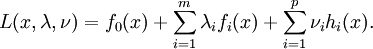
 is defined as
 and any
  . If a
  .
.