
2009. 3. 9. 15:47
@GSMC/서용덕: Convex Optimization
By Bernard Kolman, Robert Edward Beck
Contributor Robert Edward Beck
Edition: 2, illustrated
Published by Academic Press, 1995
ISBN 012417910X, 9780124179103
449 pages
Prologue
: Introduction to Operations Research
: Introduction to Operations Research
Definitions
Operations research (OR) is a scientific method for providing a quantitative basis for decision making (that can be used in almost any field of endeavor).
http://en.wikipedia.org/wiki/Operations_research
The techniques of OR give a logical and systematic way of formulating a problem so that the tools of mathematics can be applied to find a solution (when the established way of doing things can be improved.
A central problem in OR is the optimal allocation of scarce resources (including raw materials, labor, capital, energy, and processing time).
eg. T. C. Koopmans and L. V. Kantorovich, the 1975 Nobel Prize awardees
Development
WWII, Great Britain
the United States Air Force
1947, George B. Dantzig, the simplex algorithm (for solving linear programming problems)
programmable digital computer (for solving large-scale linear programming problems)
1952, the National Bureau of Standards SEAC machine
Phases
> Steps
1. Problem definition and formulation
to clarify objectives in undertaking the study
to identify the decision alternatives
to consider the limitations, restrictions, and requirement of the various alternatives
to identify the decision alternatives
to consider the limitations, restrictions, and requirement of the various alternatives
2. Model construction
to develop the appropriate mathematical description of the problem
: limitations, restrictions, and requirements -> constraints
: the goal of the study -> quantified as to be maximized or minimized
: decision alternatives -> variables
: limitations, restrictions, and requirements -> constraints
: the goal of the study -> quantified as to be maximized or minimized
: decision alternatives -> variables
3. Solution of the model
: the solution to the model need not be the solution to the original problem
4. Sensitivity analysis
to determine the sensitivity of the solution to changes in the inpuit data
: how the solution will vary with the variation in the input data
: how the solution will vary with the variation in the input data
5. Model evalution
to determine whether the answers produced by the model are realistic, acceptable and capable of implementation
6. Implementation of the study
The Structure of Mathematical Models
There are two types of mathematical models: deterministic and probabilistic.
A deterministic model will always yield the same set of output values for a given set of input values, whereas a probabilistic model will typically yield many different sets of output values according to some probability distribution.
Decision variables or unknowns
to describe an optimal allocation of the scarce resources represented by the model
Parameters
: inputs, not adjustable but exactly or approximately known
Constraints
: conditions that limit the values that the decision variables can assume
Objective function
to measures the effectiveness of the system as a function of the decision variables
: The decisin variables are to be determined so that the objective function will be optimized.
: The decisin variables are to be determined so that the objective function will be optimized.
Mathematical Techniques
mathematical programming
Mathematical models call for finding values of the decision variables that maximize or minimize the objective function subject to a system of inequality and equality constraints.
Linear programming
Integer programming
Stochastic programming
Nonlinear programming
network flow analysis
standard techniques vs. heuristic techniques (improvised for the particular problem and without firm mathematical basis)
Journals
Computer and Information Systems Abstracts Journal
Computer Journal
Decision Sciences
European Journal of Operational Research
IEEE Transactions on Automatic Control
Interfaces
International Abstracts in Operations Research
Journal of Computer and System Sciences
Journal of Research of the National Bureau of Standards
Journal of the ACM
Journal of the Canadian Operational Research Society
Management Science (published by The Institute for Management Science - TIMS)
Mathematical Programming
Mathematics in Operations Research
Naval Research Logisics (published by the Office of Naval Research - ONR)
Operational Research Quarterly
Operations Research (published by the Operations Research Society of America - ORSA)
Operations Research Letters
OR/MS Today
ORSA Journal on Computing
SIAM Journal on Computing
Transportation Science
'@GSMC > 서용덕: Convex Optimization' 카테고리의 다른 글
| SeDuMi (0) | 2009.03.11 |
|---|---|
| [Kolman & Beck] Chapter 1 Introduction to Linear Programming (0) | 2009.03.11 |
| [Boyd & Vandenberghe] Chapter 4 Convex Optimization Problems (0) | 2009.03.04 |
| [Boyd & Vandenberghe] Chapter 3 Convex Functions (0) | 2009.02.23 |
| [Boyd & Vandenberghe] Chapter 2 Convex Sets (0) | 2009.02.23 |


 lpch3_simplex_method.pdf


 for some
 .
. 
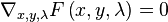
 having non-empty interior, the Lagrangian function
  is defined as
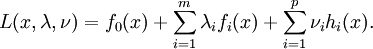
 is defined as
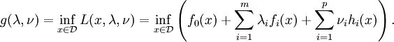
 and any
 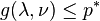 . If a
 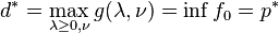 .
.