'@GSMC' 카테고리의 글 목록 (3 Page)

일	월	화	수	목	금	토
	1	2	3	4	5	6
7	8	9	10	11	12	13
14	15	16	17	18	19	20
21	22	23	24	25	26	27
28	29	30

ch.6 Multilayer Neural Networks

2008. 11. 21. 17:00 @GSMC/김경환: Pattern Recognition

SNNS (Stuttgart Neural Network Simulator)
is a software simulator for neural networks on Unix workstations developed at the Institute for Parallel and Distributed High Performance Systems (IPVR) at the University of Stuttgart. The goal of the SNNS project is to create an efficient and flexible simulation environment for research on and application of neural nets.

http://en.wikipedia.org/wiki/SNNS

Petron, E. 1999. Stuttgart Neural Network Simulator: Exploring connectionism and machine learning with SNNS. Linux J. 1999, 63es (Jul. 1999), 2.

Neural Network Toolbox™ extends MATLAB®
with tools for designing, implementing, visualizing, and simulating neural networks.

282p

6.1 Introduction

LMS (Least mean squares) algorithms

multilayer neural networks / multilayer Perceptrons
The parameters governing the nonlinear mapping are learned at the same time as those governing the linear discriminant.

http://en.wikipedia.org/wiki/Multilayer_perceptron

http://en.wikipedia.org/wiki/Neural_network

the number of layers of units
(eg. the two-layer networks = single layer networks)

Multilayer neural networks implement linear discriminants, but in a space where the inputs have been mapped nonlinearly.

backpropagation algorithm / generalized delta rule
: a natural extension of the LMS algorithm
- the intuitive graphical representation & the simplicity of design of models
- the conceptual and algorithmic simplicity

network architecture / topology
- neural net classification
- heuristic model selection (through choices in the number of hidden layers, units, feedback connections, and so on.

regularization
= complexity adjustment

284p

6.2 Feedforward Operation and Classification

http://en.wikipedia.org/wiki/Artificial_neural_network

bias unit
the function of units : "neurons"
the input units : the components of a feature vector
signals emiited by output units : the values of the discriminant functions used for classification
hidden units : the weighted sum of its inputs

-> net activation : the inner product of the inputs with the weights at the hidden unit

the input-to-hidden layer weights : "synapses" -> "synaptic weights"

activation function : "nonlinearity" of a unit

"Each hidden unit emits an output that is a nonlinear function of its activation."

"Each ouput unit computes its net activation based on the hidden unit signals."

http://en.wikipedia.org/wiki/Feedforward_neural_network

286p
6.2.1 General Feedforward Operation

"Given sufficient number of hidden units of a general type, any function can be so represented." -> expressive power

287p
6.2.2 Expressive Power of Multilayer Networks

"Any desired function can be implemented by a three-layer network."
-> but, the problems of designing and training neural networks

288p

6.3 Backpropagation Algorithm

http://en.wikipedia.org/wiki/Backpropagation

- the problem of setting the weights (based on training patterns and the desired output)
- supervised training of multilayer neural networks
- the natural extension of the LMS algorithm for linear systems
- based on gradient descent

credit assignment problem
: no explicit teacher to state what the hidden unit's output should be

=> The power of backpropagation to calculate an effective error for each hidden unit, and thus derive a learning rule for the input-to-hidden weights

sigmoid

6.3.1 Network Learning

The final signals emitted by the network are used as discriminant functions for classification. During network training, these output signals are compared with a teaching or target vector t, and any difference is used in training the weights throughout the network

training error -> LMS algorithm
gradient descent -> the weights are changed in a direction that will reduce the error

6.3.2 Training Protocol

6.3.3 Learning Curves

6.4 Error Surfaces

6.8.1 Activation Function

'@GSMC > 김경환: Pattern Recognition' 카테고리의 다른 글

ch.7 Stochastic Methods (0)	2008.12.03
ch.5 Linear Discriminant Functions (0)	2008.11.02
ch.4 Nonparametric Techniques (0)	2008.10.21
ch.3 Maximum-Likelihood and Bayesian Parameter Estimation (0)	2008.10.08
ch.2 Bayesian Decision Theory (0)	2008.09.25

posted by maetel

ch.5 Linear Discriminant Functions

2008. 11. 2. 16:51 @GSMC/김경환: Pattern Recognition

215p

5.1 Introduction

http://en.wikipedia.org/wiki/Statistical_classification

http://en.wikipedia.org/wiki/Linear_classifier

http://en.wikipedia.org/wiki/Linear_discriminant_analysis

linear discriminant functions
1) linear in the components of a feature vector
2) linear in some given set of functions of a feature vector

finding a linear discriminant function
-> minimizing a criterion fuction - sample risk / training error
: "A small training error does not guarantee a small test error."
=> to derive the minimum-risk linear discriminant

-> "convergence properties & computational complexities" of gradient descent procedures for minimizing criterion functions

216p

5.2 Linear Discriminant Functions and Decision Surfaces

weight vector
bias / threshold weight

5.2.1 The Two-Category Case

"The effective input is the sum of each input feauture value multiplied by its corresponding weight."

http://en.wikipedia.org/wiki/Hyperplane

"The weight vector is normal to any vector lying in the hyperplane."

A linear discriminant function divides the feature space by a hyperplane decision surface.

The orientation of the surface is determined by the normal vector w.
The location of the surface is determined by the bias w_0.

The discriminant function g(x) is proportional to the signed distance from x to the hyperplane.

218p
5.2.2 The Multicategory Case

A linear machine divides the feature space into c decision regions.

If the decision regions are contiguous, the boundary between them is a portion of the hyperplane.

With the linear machine, the decision boundary is determined by the differences of the weight vectors.

There are c(c-1)/2 paris of regions.

The linear machines are most suitable for problems for which the conditional densities are unimodal.

219p

5.3 Generalized Linear Discriminant Functions

quadratic discriminant function
2008/11/05 - [Method/Nature] - Jonathan Richard Shewchuk - An Introduction to the Conjugate Gradient Method Without the Agonizing Pain

http://en.wikipedia.org/wiki/Quadratic_classifier

http://en.wikipedia.org/wiki/Quadric

The separating surface defined by the quadratic discriminant function is a second-degree or hyperquadric surface.

http://en.wikipedia.org/wiki/Hypersphere
http://en.wikipedia.org/wiki/Hyperboloid

http://en.wikipedia.org/wiki/Scaling_(geometry )
if the scaled matrix is
i) the positive multiple of the identity matrix
    => hypershere
ii) positive definete
    => hyperellipsoid
iii) some of eigenvalues of it are positive and others negative
    => various hyperhyperboloids
==> general multivariate Gaussian case

polynomial discriminant function
-> generalized linear discriminant function
: not linear in the feature vector x but linear in arbitrary functions y (phi function) of x

The mapping from x-space to y-space comes to find a homogeneous linear discriminant function.

Even with relatively simple functions y(x), decision surfaces induced in an x-space can be fairly complex.

the curse of dimensionality
-> the number of samples should be not less than the number of degrees of freedom. (-> ch.9)

http://en.wikipedia.org/wiki/Big_O_notation

http://en.wikipedia.org/wiki/Margin_(machine_learning)
The margin of a single data point is defined to be the distance from the data point to a decision boundary.
cf. VC dimension Tutorial Slides by Andrew Moore

http://en.wikipedia.org/wiki/Artificial_neural_network

http://en.wikipedia.org/wiki/Multilayer_perceptron

augmented feature vector, y
augmented weight vector, a

The hyperplane desicion surface in y-space passes through the origin in y-space.

The mapping from d-dim x-space to (d+1)-dim y-space preserves all distance relationships among samples.
-> The distance from y to the transformed hyperplane is less than or equal to the distance from x to the original hyperplane.

223p

5.4 The Two-Category Linearly Separable Case

separating vector / solution vector (to normalize samples in the feature space)

http://en.wikipedia.org/wiki/Weight_(representation_theory )

5.4.1 Geometry and Terminology

The linear discriminant equation defines a hyperplane through the origin of weight space having y_i as a normal vector.

The solution vector must be on the positivie side of every hyperplane and lie in the intersection of n half-spaces. -> solution region

-> To find a solution vector closer to the "middle" of the solution region
-> margin

224p
5.4.2 Gradient Descent Procedures

To define a criterion function J(a) that is minimized if a is a solution vector

(1) BGD = Basic Gradient Descent
The next weight vector is obtained by moving some distance from the former one in the direction of steepest descent, along the negative of the gradient of a criterion function.

(2) Newton's algorithm
- To minimize the second-order expansion for the quadratic error functions
- To leads to greater improvement per step
- computational burden of inverting the Hessian matrix

learning rate (to set the step size)

http://en.wikipedia.org/wiki/Gradient_descent
The (negative) gradient at a point is orthogonal to the contour line going through that point.

http://en.wikipedia.org/wiki/Hessian_matrix

http://en.wikipedia.org/wiki/Taylor_series
The Taylor series is a representation of a function as an infinite sum of terms calculated from the values of its derivatives at a single point.
(As the degree of the Taylor polynomial rises, it approaches the correct function.

http://en.wikipedia.org/wiki/Newton%27s_method

http://en.wikipedia.org/wiki/Quasi-Newton_method

227p

5.5 Minimizing The Perception Criterion Function

5.5.1 The Perceptron Criterion Function

http://en.wikipedia.org/wiki/Perceptron

Perceptron criterion function
- never negative, being zero only if a is a solution vector or if a is on the decision boundary.
- propotional to the sum of the distances from the misclassified samples to the decision boundary

Perceptron criterion is piecewise linear and acceptable for gradient descent.

batch training
batch Perceptron algorithm:
The next weight vector is obtained by adding some multiple of the sum of the misclassified samples to the present weight vector.

229p
5.5.2 Convergence Proof for Single-Sample Correction

http://en.wikipedia.org/wiki/Convergence_of_random_variables

We shall modify the weight vector whenever it misclassifies a single sample.
For the purposes of the convergence proof, repeat the samples cyclically.
: We must store and revisit all of the training patterns.
: We shall only change the weight vector when there is an error

Fixed-Increment Single-Sample Perceptron
The correction is moving the weight vector in a good direction, until the samples are linearly separable.

Fig.5.13
A correction which is proportional to the pattern vector is added to the weight vector.
Each correction brings the weight vector closer to the solution region.

Theorem 5.1. Perceptron Convergence
If training samples are linearly separable, then the sequence of weight vectors given by Fixed-Increment Single-Sample Perceptron algorithm will terminate at a solution vector.

232p
5.5.3 Some Direct Generalizations

Algorithm 5: Variable-Increment Percceptron with Margin
correction with a variable increment and a margin

Algorithm 6: Batch Variable Increment Perceptron
the trajectory of the weight vector is smoothed

Algorithm 7: Balanced Winnow
for separable data the gap determined by the two contituent weight vectors can naver increase in size. -> a convergence proof
http://en.wikipedia.org/wiki/Winnow_(algorithm)

235p

5.6 Relaxation Procedures

5.6.1 The Descent Algorithm

a squared error function:
- The gradient is countinuous(, whereas the gradient of a Perceptron criterion function is not.)
- to search a smoother surface
- so smoother near the boundary of the solution region (that the sequence of weight vectors can converge to a point on the boundary)
- the gradient reaches the boundary point when the weight vector is zero vector
- dominated by the longest sample vectors

a squared error with margin:
- never negative, (zero iff weighted samples misclassified by the weight is equal to or more than the margin)

Algorithm 8: Batch Relaxation with Margin

Algorithm9: Single-Sample Relaxation with Margin

relaxation
under-relaxation
over-relaxation

237p
5.6.2 Convergence Proof

238p

5.7 Nonseparable Behavior

error-correcting procedures to call for a modification of the weight vector when and only when an error is encountered

The length of the weight vectors produced by the fixed-increment rule are bounded (, fluctuating near some limiting value).

If the components of the samples are integer-valued, the fixed-increment procedure yields a finite-state process.

Averaging the weight vectors can reduce the risk of obtaining a bad solution.

5.8 Minimum Squared-error Procedures

5.8.4 The Widrow-Hoff or LMS Procedure

http://en.wikipedia.org/wiki/Least_mean_squares_filter

5.8.5 Stochastic Approximation Methods

http://en.wikipedia.org/wiki/Stochastic_gradient_descent

5.9 The Ho-Koshyap Procedures

5.11 Support Vector Machines

5.12 Multicategory Generalizations

5.12.1 Kesler's construction

to convert many multicategory error-correction procedures to two-category procedures for the purpose of obtaining a convergence proof

5.12.2 Convergence of the Fixed-Increment Rule

5.12.3 Generalizaions for MSE Procedures

'@GSMC > 김경환: Pattern Recognition' 카테고리의 다른 글

ch.7 Stochastic Methods (0)	2008.12.03
ch.6 Multilayer Neural Networks (0)	2008.11.21
ch.4 Nonparametric Techniques (0)	2008.10.21
ch.3 Maximum-Likelihood and Bayesian Parameter Estimation (0)	2008.10.08
ch.2 Bayesian Decision Theory (0)	2008.09.25

posted by maetel

Lecture 8: Uncalibrated Multiple-View Geometry: Fundamental Matrix

2008. 10. 28. 09:00 @GSMC/이상욱: Principles of Human and Artificial Vision

Fundamental Matrix

http://en.wikipedia.org/wiki/Fundamental_matrix_(computer_vision)
In computer vision, the fundamental matrix $\mathbf{F}$ is a $3 \times 3$ matrix of rank 2 which relates corresponding points in stereo images. In epipolar geometry, with homogeneous image coordinates $\mathbf{y_1}$ and $\mathbf{y_2}$ of corresponding points in a stereo image pair, $\mathbf{F y_1}$ describes a line (an epipolar line) on which the corresponding point $y 2$ on the other image must lie. That means, for all pairs of corresponding points holds

$\mathbf{ y_2^T F y_1} = 0.$

Being of rank two and determined only up to scale, the fundamental matrix can be estimated given at least seven point correspondences. Its seven parameters represent the only geometric information about cameras that can be obtained through point correspondences alone.

epipole
epipolar line
epipolar plane

http://en.wikipedia.org/wiki/Epipolar_geometry

RANdom SAmple Consensus
http://en.wikipedia.org/wiki/RANSAC

ref.
http://www.robots.ox.ac.uk/~vgg/hzbook/index.html

http://nonsense.danielwedge.com/2008/10/19/the-fundamental-matrix-song/

An Invitation to 3-D Vision
Yi Ma, Stefano Soatto, Jana Kosecka, Shankar Sastry
Springer Verlag, 2003

Learning Epipolar Geometry
The Java code for this page was created by Sylvain Bougnoux.

'@GSMC > 이상욱: Principles of Human and Artificial Vision' 카테고리의 다른 글

Lecture 10: Uncalibrated Multi-view Geometry - Reconstruction (0)	2008.12.04
Lecture 9: Multi-view Geometry (0)	2008.12.04
Lecture 7: Image Filtering & Edge Detection (0)	2008.10.28
Lecture 6: Multiple-View Geometry: Stereo, Motion, Features (0)	2008.10.27
Lecture 5: Single Camera View Geometry (0)	2008.10.27

posted by maetel

Lecture 7: Image Filtering & Edge Detection

2008. 10. 28. 03:00 @GSMC/이상욱: Principles of Human and Artificial Vision

image filtering
image warping

LSI (Linear Shift Invariance) - convolution

http://en.wikipedia.org/wiki/Convolution
Convolution is a mathematical operation on two functions f and g, producing a third function that is typically viewed as a modified version of one of the original functions.

http://en.wikipedia.org/wiki/Cross_correlation

http://en.wikipedia.org/wiki/Gaussian_filter
Mathematically, a Gaussian filter modifies the input signal by convolution with a Gaussian function; this transformation is also known as the Weierstrass transform.
Gaussian filters are designed to give no overshoot to a step function input while minimizing the rise and fall time (which leads to the steepest possible slope). This behavior is closely connected to the fact that the Gaussian filter has the minimum possible group delay.

'@GSMC > 이상욱: Principles of Human and Artificial Vision' 카테고리의 다른 글

Lecture 9: Multi-view Geometry (0)	2008.12.04
Lecture 8: Uncalibrated Multiple-View Geometry: Fundamental Matrix (0)	2008.10.28
Lecture 6: Multiple-View Geometry: Stereo, Motion, Features (0)	2008.10.27
Lecture 5: Single Camera View Geometry (0)	2008.10.27
Lecture 4: Projective Geometry (0)	2008.10.26

posted by maetel

Lecture 6: Multiple-View Geometry: Stereo, Motion, Features

2008. 10. 27. 22:48 @GSMC/이상욱: Principles of Human and Artificial Vision

Structure from Stereo

two or more images, calibrated cameras (K(f), R, T known)
http://en.wikipedia.org/wiki/Stereo_vision

ref.
UCR stereographs
http://www.cmp.ucr.edu/site/exhibitions/stereo/
The Art of Stereo Photography
http://www.photostuff.co.uk/stereo.htm
History of Stereo Photography
http://www.rpi.edu/~ruiz/stereo_history/text/historystereog.html
Double Exposure
http://home.centurytel.net/s3dcor/index.html
Stereo Photography
http://www.shortcourses.com/book01/chapter09.htm
3D Photography links
http://www.studyweb.com/links/5243.html
National Stereoscopic Association
http://204.248.144.203/3dLibrary/welcome.html
Books on Stereo Photography
http://userwww.sfsu.edu/~hl/3d.biblio.html

http://en.wikipedia.org/wiki/Epipolar_geometry

http://en.wikipedia.org/wiki/Image_rectification
http://en.wikipedia.org/wiki/Rectification_(geometry)

Computing Rectifying Homographies for Stereo Vision
Charles Loop, Zhengyou Zhang

ComputingRectifyingHomographies.pdf

Microsoft Research, April 8, 1999

cross correlation
http://en.wikipedia.org/wiki/Cross_correlation

S. M. Seitz and C. R. Dyer, View Morphing, Proc. SIGGRAPH 96, 1996, pp. 21-30.

L. McMillan and G. Bishop. Plenoptic Modeling: An Image-Based Rendering System, Proc. of SIGGRAPH 95, 1995, pp. 39-46.

> Stereo Reconstruction
1) Calibrate cameras
2) Rectify images
3) Compute disparity
4) Estimate depth

SSD (Sum of Squared Difference) to choose the baseline

Structure from Motion

Incremental Motion: Kinematic relation

7 Unknowns respect to motion
translation: V = (VX , VY , VZ )
rotation :     W = (WX, WY, WZ )
depth :         Z
2 equations for one point

6 points with 12 unknowns -> 12 equations

http://en.wikipedia.org/wiki/Structure_from_motion
http://en.wikipedia.org/wiki/Motion_field

http://en.wikipedia.org/wiki/Nodal_point#Nodal_points

optical flow, image flow
http://en.wikipedia.org/wiki/Optical_flow

Horn-Schunck Algorithm
http://en.wikipedia.org/wiki/Horn-Schunck_algorithm

Determining Optical Flow

horn_schunck_DeterminingOpticalFlow.pdf

Berthold K.P. Horn and Brian G. Schunck
Artificial Intelligence Laboratory, Massachusetts Institute of Technology

Larger Motion - feature matching

Lucas Kanade style motion estimation
http://en.wikipedia.org/wiki/Lucas%E2%80%93Kanade_method

Good Features to Track

shi_tomasi_GoodFeaturesToTrack.pdf

Jianbo Shi (Computer Science Department, Cornel1 University)
Carlo Tomasi (Computer Science Department, Stanford University)

http://en.wikipedia.org/wiki/Kalman_filter

'@GSMC > 이상욱: Principles of Human and Artificial Vision' 카테고리의 다른 글

Lecture 8: Uncalibrated Multiple-View Geometry: Fundamental Matrix (0)	2008.10.28
Lecture 7: Image Filtering & Edge Detection (0)	2008.10.28
Lecture 5: Single Camera View Geometry (0)	2008.10.27
Lecture 4: Projective Geometry (0)	2008.10.26
Lecture 3: Linear Algebra for Computer Vision (0)	2008.10.26

posted by maetel

Lecture 5: Single Camera View Geometry

2008. 10. 27. 03:48 @GSMC/이상욱: Principles of Human and Artificial Vision

cross ratio
http://en.wikipedia.org/wiki/Cross_ratio
http://www.mathpages.com/home/kmath543/kmath543.htm
http://www.cut-the-knot.org/pythagoras/Cross-Ratio.shtml

measuring height: algebraic derivation from the cross ratio

Planar Perspective Map (homography) H
H Maps reference plane X-Y coordinates to image plane x-y coordinates
Fully determined from 4 known points on ground plane
Option A: physically measure 4 points on ground
Option B: find a square, guess the size
Option C: Note H = [avX bvY l] (columns 1,2,4 of P )
Play with scale factors a and b until the model “looks right”
Given x-y , can find X-Y by H-1 :

To compute camera projection matrix, we can measure

- Positions within a plane
- Height (More generally — distance between any two parallel planes)
- Camera position

Single View Metrology

criminisi_reid_zisserman_SingleViewMetrology.pdf

A. Criminisi, I. Reid and A. Zisserman
Department of Engineering Science, University of Oxford

> Assumptions
1)   3 orthogonal sets of parallel lines
2)   4 known points on ground plane
3)   1 height in the scene

> Complete approach
- Load in an image
- Click on parallel lines defining X, Y, and Z directions
- Compute vanishing points
- Specify points on reference plane, ref. height
- Compute 3D positions of several points
- Create a 3D model from these points
- Extract texture maps
- Output a VRML model

http://en.wikipedia.org/wiki/VRML
VRML (Virtual Reality Modeling Language, pronounced vermal or by its initials, originally — before 1995 — known as the Virtual Reality Markup Language) is a standard file format for representing 3-dimensional (3D) interactive vector graphics, designed particularly with the World Wide Web in mind. It has been superseded by X3D.

3-D Metrology
http://research.microsoft.com/~antcrim/

single view reconstruction

http://en.wikipedia.org/wiki/Ground_truth

radial distortion
http://en.wikipedia.org/wiki/Distortion_(optics)

'@GSMC > 이상욱: Principles of Human and Artificial Vision' 카테고리의 다른 글

Lecture 7: Image Filtering & Edge Detection (0)	2008.10.28
Lecture 6: Multiple-View Geometry: Stereo, Motion, Features (0)	2008.10.27
Lecture 4: Projective Geometry (0)	2008.10.26
Lecture 3: Linear Algebra for Computer Vision (0)	2008.10.26
Lecture 2: Image Formation & Camera Calibration (0)	2008.10.24

posted by maetel

Lecture 4: Projective Geometry

2008. 10. 26. 23:13 @GSMC/이상욱: Principles of Human and Artificial Vision

plane projective transformation
(Z_w = 0 -> 3-by-3 matrix representing a general plane to plane projective transformation)
http://en.wikipedia.org/wiki/Projective_plane

rotation about the optical center
: depth-independent transformation
(H does not depend on 3D structure.)

synthetic rotations
projective warping
http://en.wikipedia.org/wiki/Image_warping

null space
http://en.wikipedia.org/wiki/Kernel_(matrix)
The null space of a matrix with n columns is a linear subspace of n-dimensional Euclidean space.
The null space of A is the same as the solution set to the homogeneous system.
(cf. http://en.wikipedia.org/wiki/Kernel_(mathematics)
http://en.wikipedia.org/wiki/Kernel_(linear_operator) )

> 2d transformation
- Euclidian transformation
- affine transformation
http://en.wikipedia.org/wiki/Affine_transformation
- similarity transformation
http://en.wikipedia.org/wiki/Similarity_transformation
- projective transformation
http://en.wikipedia.org/wiki/Projective_transformation

> projective plane
homography
http://en.wikipedia.org/wiki/Homography

homogeneous coordinates
http://en.wikipedia.org/wiki/Homogeneous_coordinate

perspective projection
http://en.wikipedia.org/wiki/Perspective_projection#Perspective_projection

projective space
http://en.wikipedia.org/wiki/Projective_space

A point in the image is a ray in projective space.

=> All points on the ray are equivalent.

3D Projective Geometry

These concepts generalize naturally to 3D
- Homogeneous coordinates
Projective 3D points have four coords: X = (X,Y,Z,W)
- Duality
A plane L is also represented by a 4-vector
Points and planes are dual in 3D: LTP = 0
- Projective transformations
Represented by 4x4 matrices T: X’ = TX, X’ = L X -1

However
- Can’t use cross-products in 4D. We need new tools
Grassman-Cayley Algebra
: generalization of cross product, allows interactions between points, lines, and planes via “meet” and “join” operators
- Or just use inhomogeneous representation in 3D.

http://en.wikipedia.org/wiki/Grassman_algebra

vanishing point
http://mathdl.maa.org/mathDL/1//?pa=content&sa=viewDocument&nodeId=477&bodyId=598

vanishing line

http://en.wikipedia.org/wiki/Perspective_(graphical)

'@GSMC > 이상욱: Principles of Human and Artificial Vision' 카테고리의 다른 글

Lecture 7: Image Filtering & Edge Detection (0)	2008.10.28
Lecture 6: Multiple-View Geometry: Stereo, Motion, Features (0)	2008.10.27
Lecture 5: Single Camera View Geometry (0)	2008.10.27
Lecture 3: Linear Algebra for Computer Vision (0)	2008.10.26
Lecture 2: Image Formation & Camera Calibration (0)	2008.10.24

posted by maetel

Lecture 3: Linear Algebra for Computer Vision

2008. 10. 26. 21:32 @GSMC/이상욱: Principles of Human and Artificial Vision

'@GSMC > 이상욱: Principles of Human and Artificial Vision' 카테고리의 다른 글

Lecture 7: Image Filtering & Edge Detection (0)	2008.10.28
Lecture 6: Multiple-View Geometry: Stereo, Motion, Features (0)	2008.10.27
Lecture 5: Single Camera View Geometry (0)	2008.10.27
Lecture 4: Projective Geometry (0)	2008.10.26
Lecture 2: Image Formation & Camera Calibration (0)	2008.10.24

posted by maetel

Lecture 2: Image Formation & Camera Calibration

2008. 10. 24. 19:40 @GSMC/이상욱: Principles of Human and Artificial Vision

http://en.wikipedia.org/wiki/Pinhole_camera
Cameras using small apertures, and the human eye in bright light both act like a pinhole camera. The smaller the hole, the sharper the image, but the dimmer the projected image. Optimally, the size of the aperture, should be 1/100 or less of the distance between it and the screen.

http://en.wikipedia.org/wiki/Projection_matrix
a projection is a linear transformation P from a vector space to itself such that P2 = P. It leaves its image unchanged. Though abstract, this definition of "projection" formalizes and generalizes the idea of graphical projection.

http://en.wikipedia.org/wiki/Orthographic_projection
Increasing the focal length and distance of the camera to infinity in a perspective projection results in an orthographic projection. It is a form of parallel projection, where the view direction is orthogonal to the projection plane.

http://en.wikipedia.org/wiki/Homogeneous_coordinate
The homogeneous coordinates of a point of projective space of dimension n are usually written as (x : y : z : ... : w), a row vector of length n + 1, other than (0 : 0 : 0 : ... : 0). Two sets of coordinates that are proportional denote the same point of projective space: for any non-zero scalar c from the underlying field K, (cx : cy : cz : ... : cw) denotes the same point. Therefore this system of coordinates can be explained as follows: if the projective space is constructed from a vector space V of dimension n + 1, introduce coordinates in V by choosing a basis, and use these in P(V), the equivalence classes of proportional non-zero vectors in V.

http://en.wikipedia.org/wiki/Affine_transformation
In geometry, an affine transformation or affine map or an affinity (from the Latin, affinis, "connected with") between two vector spaces (strictly speaking, two affine spaces) consists of a linear transformation followed by a translation:
$x \mapsto A x+ b$
In the finite-dimensional case each affine transformation is given by a matrix A and a vector b, satisfying certain properties described below.
Physically, an affine transformation is one that preserves

1. Collinearity between points, i.e., three points which lie on a line continue to be collinear after the transformation
2. Ratios of distances along a line, i.e., for distinct colinear points p1, p2, p3, the ratio | p2 − p1 | / | p3 − p2 | is preserved

In general, an affine transform is composed of zero or more linear transformations (rotation, scaling or shear) and a translation (or "shift"). Several linear transformations can be combined into a single matrix, thus the general formula given above is still applicable.

http://en.wikipedia.org/wiki/Projective_space
The idea of a projective space relates to perspective, more precisely to the way an eye or a camera projects a 3D scene to a 2D image. All points which lie on a projection line (i.e. a "line-of-sight"), intersecting with the focal point of the camera, are projected onto a common image point. In this case the vector space is R3 with the camera focal point at the origin and the projective space corresponds to the image points.
( For example, in the standard geometry for the plane two lines always intersect at a point except when the lines are parallel. In a projective representation of lines and points, however, such an intersection point exists even for parallel lines, and it can be computed in the same way as other intersection points. )

http://en.wikipedia.org/wiki/Projective_geometry
Projective geometry is the most general and least restrictive in the hierarchy of fundamental geometries, i.e. Euclidean - metric (similarity) - affine - projective. It is an intrinsically non-metrical geometry, whose facts are independent of any metric structure. Under the projective transformations, the incidence structure and the cross-ratio are preserved. It is a non-Euclidean geometry. In particular, it formalizes one of the central principles of perspective art: that parallel lines meet at infinity and therefore are to be drawn that way. In essence, a projective geometry may be thought of as an extension of Euclidean geometry in which the "direction" of each line is subsumed within the line as an extra "point", and in which a "horizon" of directions corresponding to coplanar lines is regarded as a "line". Thus, two parallel lines will meet on a horizon line in virtue of their possessing the same direction.

http://en.wikipedia.org/wiki/Camera_resectioning
When a camera is used, light from the environment is focused on an image plane and captured. This process reduces the dimensions of the data taken in by the camera from three to two (light from a 3D scene is stored on a 2D image). Each pixel on the image plane therefore corresponds to a shaft of light from the original scene. Camera resectioning determines which incoming light is associated with each pixel on the resulting image.

http://en.wikipedia.org/wiki/Camera_matrix
Since the camera matrix is involved in the mapping between elements of two projective spaces, it too can be regarded as a projective element. This means that it has only 11 degrees of freedom since any multiplication by a non-zero scalar results in an equivalent camera matrix.

http://en.wikipedia.org/wiki/Euclidean_space
An n-dimensional space with notions of distance and angle that obey the Euclidean relationships is called an n-dimensional Euclidean space.
An essential property of a Euclidean space is its flatness. Other spaces exist in geometry that are not Euclidean.

http://en.wikipedia.org/wiki/Euclidean_transformation
The Euclidean group E(n) is a subgroup of the affine group for n dimensions, and in such a way as to respect the semidirect product structure of both groups.
1. by a pair (A, b), with A an n×n orthogonal matrix, and b a real column vector of size n; or
2. by a single square matrix of size n + 1, as explained for the affine group.

http://en.wikipedia.org/wiki/Orthogonal_matrix
$Q^T Q = Q Q^T = I . \,\!$

http://en.wikipedia.org/wiki/Singular_value_decomposition

$M = U\Sigma V^*, \,\!$

where U is an m-by-m unitary matrix over K, the matrix Σ is m-by-n diagonal matrix with nonnegative numbers on the diagonal, and V* denotes the conjugate transpose of V, an n-by-n unitary matrix over K. Such a factorization is called a singular-value decomposition of M.

The matrix V thus contains a set of orthonormal "input" or "analysing" basis vector directions for M
The matrix U contains a set of orthonormal "output" basis vector directions for M
The matrix Σ contains the singular values, which can be thought of as scalar "gain controls" by which each corresponding input is multiplied to give a corresponding output.

A common convention is to order the values Σ_i,i in non-increasing fashion. In this case, the diagonal matrix Σ is uniquely determined by M (though the matrices U and V are not).

http://en.wikipedia.org/wiki/Total_least_squares
total least squares = errors in variables = rigorous least squares = orthogonal regression

http://en.wikipedia.org/wiki/RQ_decomposition#Relation_to_RQ_decomposition

'@GSMC > 이상욱: Principles of Human and Artificial Vision' 카테고리의 다른 글

Lecture 7: Image Filtering & Edge Detection (0)	2008.10.28
Lecture 6: Multiple-View Geometry: Stereo, Motion, Features (0)	2008.10.27
Lecture 5: Single Camera View Geometry (0)	2008.10.27
Lecture 4: Projective Geometry (0)	2008.10.26
Lecture 3: Linear Algebra for Computer Vision (0)	2008.10.26

posted by maetel

ch.4 Nonparametric Techniques

2008. 10. 21. 19:09 @GSMC/김경환: Pattern Recognition

161p

4.1 Introduction

nonparametric procedures (with arbitrary distribution and without the assumption that the forms of the underlying densities are known)

1) estimating the density functions from sample patterns -> designing the classfier
2) directly estimating the a posteriori probability -> the nearest-neighbor rule -> decision functions

4.2 Density Estimation

http://en.wikipedia.org/wiki/Density_estimation
the construction of an estimate, based on observed data, of an unobservable underlying probability density function. The unobservable density function is thought of as the density according to which a large population is distributed; the data are usually thought of as a random sample from that population

i.i.d. = Independent and identically-distributed random variables
http://en.wikipedia.org/wiki/Iid
In probability theory, a sequence or other collection of random variables is independent and identically distributed (i.i.d.) if each has the same probability distribution as the others and all are mutually independent.

http://en.wikipedia.org/wiki/Binomial_coefficient
$\tbinom nk$ is the number of k-element subsets (the k-combinations) of an n-element set; that is, the number of ways that k things can be 'chosen' from a set of n things.

http://en.wikipedia.org/wiki/Probability_density_function
a function that represents a probability distribution in terms of integrals

kernel density estimation; Parzen window method
http://en.wikipedia.org/wiki/Parzen_window
a non-parametric way of estimating the probability density function of a random variable.
Given some data about a sample of a population, kernel density estimation makes it possible to extrapolate the data to the entire population.

http://en.wikipedia.org/wiki/Kernel_(statistics)
A kernel is a weighting function used in non-parametric estimation techniques. Kernels are used in kernel density estimation to estimate random variables' density functions, or in kernel regression to estimate the conditional expectation of a random variable.

http://en.wikipedia.org/wiki/Hypercube

http://en.wikipedia.org/wiki/Neural_networks

'@GSMC > 김경환: Pattern Recognition' 카테고리의 다른 글

ch.6 Multilayer Neural Networks (0)	2008.11.21
ch.5 Linear Discriminant Functions (0)	2008.11.02
ch.3 Maximum-Likelihood and Bayesian Parameter Estimation (0)	2008.10.08
ch.2 Bayesian Decision Theory (0)	2008.09.25
Pattern Classification: ch.1 Introduction (0)	2008.09.03

posted by maetel

2.4 Color images & 2.5 Cameras

2008. 10. 16. 20:42 @GSMC/박래홍: Computer Vision

2.4 Color images

2.4.1 Physics of color

2.4.2 Color perceived by humans

XYZ color space
http://en.wikipedia.org/wiki/Xyz_color_space

color matching functions
: numerical description of the chromatic response of the observer

color gamut:
subsapce of colors perceived by humans

http://en.wikipedia.org/wiki/Gamut
Digitizing a photograph, converting a digitized image to a different color space, or outputting it to a given medium using a certain output device generally alters its gamut, in the sense that some of the colors in the original are lost in the process.

37p

2.4.3 Color spaces

http://en.wikipedia.org/wiki/Color_space

http://en.wikipedia.org/wiki/Rounding_error

(1) RGB color space
- CRT
- relative color standard
- additive color mixing
- sRGB, Adobe RGB, Adobe Wide Gamut RGB

http://en.wikipedia.org/wiki/RGB_color_space
The complete specification of an RGB color space also requires a white point chromaticity and a gamma correction curve.

(2) YIQ color space

- additive color mixing
- luminance (the perceived energy ot a light source)

http://en.wikipedia.org/wiki/YIQ
The Y component represents the luma information, and is the only component used by black-and-white television receivers. I and Q represent the chrominance information.

(3) YUV color space

http://en.wikipedia.org/wiki/YUV
Y' stands for the luma component (the brightness) and U and V are the chrominance (color) components.

(4) CMY color space
- subtractive color mixing (in printing process)
- sets of inks, substrates, and press characteristics

http://en.wikipedia.org/wiki/CMYK_color_model
masking certain colors on the typically white background (that is, absorbing particular wavelengths of light)

(5) HSV color space
- Hue, Saturation, Value (; HSB, Hue, Saturation, Brightness ; HSI; Hue, Saturation, Intensity)
- => image enhancement algorithms

http://en.wikipedia.org/wiki/HSL_and_HSV
Because HSL and HSV are simple transformations of device-dependent RGB, the color defined by a (h, s, l) or (h, s, v) triplet depends on the particular color of red, green, and blue “primaries” used. Each unique RGB device therefore has unique HSL and HSV spaces to accompany it. An (h, s, l) or (h, s, v) triplet can however become definite when it is tied to a particular RGB color space, such as sRGB.

39p

2.4.4 Palette images

palette images; indexed images

lookup table; color table; color map; index register; palette

The number of colors in the image exceeds the number of entries in the lookup table and a subset of colors has to be chosen, and a loss of information occurs.

http://en.wikipedia.org/wiki/Palette_(computing)

http://en.wikipedia.org/wiki/List_of_palettes

http://en.wikipedia.org/wiki/Indexed_color

vector quantization (-> 14.4)
1) to check which colors appear in the image by creating histograms for all three color components
2) to quantize them to provide more shades for colors which occur in the image frequently
3) to find the nearest color in the lookup table to represent the color

=> to analyze large multi-dimensional datasets

http://en.wikipedia.org/wiki/Vector_quantization

http://en.wikipedia.org/wiki/Cluster_analysis
Clustering is the classification of objects into different groups, or more precisely, the partitioning of a data set into subsets (clusters), so that the data in each subset (ideally) share some common trait - often proximity according to some defined distance measure.

http://en.wikipedia.org/wiki/K_means
The k-means algorithm is an algorithm to cluster n objects based on attributes into k partitions, k < n. It is similar to the expectation-maximization algorithm for mixtures of Gaussians in that they both attempt to find the centers of natural clusters in the data.

pseudocolor

Palette selection depends on the semantics of the image and is an interactive process.

2.4.5 Color constancy

The same surface color under diffrent illumination

von Kries coefficients
http://en.wikipedia.org/wiki/Color_vision

> color compensations

- to scale the sensitivity of each sensor type

=> automatic white balancing

- to assume that the brightest point in the image has the color of the illumination

2.5 Cameras: an overview

2.5.1 Photosensitive sensors

> photosensitive sensors in cameras
(1) photo-emission

photoelectric effect (; Hertz Effect)
http://en.wikipedia.org/wiki/Photoelectric_effect

photomultipliers
vacuum tube TV cameras

(2) photovoltanic

http://en.wikipedia.org/wiki/Solar_cell

photodiode
night vision camera
photoresistor
Schottky photodiode

> semiconductor photoresistive sensors
(1) CCDs (charge-coupled devices)
- arranged into a matrix-like grid of pixels (CCD chip)
- blooming effect
- shift registers
- SNR fropped

(2) CMOS (complementary metal oxide semiconductor)
- all of the pixel area devoted to light capture
- matrix-like sensors

2.5.2 A monochromatic camera

2.5.3 A color camera

2.6 Summary

'@GSMC > 박래홍: Computer Vision' 카테고리의 다른 글

Ch.10 Image Understanding (0)	2008.12.15
Ch.9 Object Recognition (0)	2008.11.25
Ch. 6 Segmentation I (0)	2008.09.20
Ch. 2 The image, its representations and properties (0)	2008.09.10
Ch.1 Introduction (0)	2008.09.04

posted by maetel

ch.3 Maximum-Likelihood and Bayesian Parameter Estimation

2008. 10. 8. 20:06 @GSMC/김경환: Pattern Recognition

3.2 Maximum-Likelihood Estimation

maximum-likelihood

http://en.wikipedia.org/wiki/Maximum_likelihood

a popular statistical method used for fitting a mathematical model to some data. The modeling of real world data using estimation by maximum likelihood offers a way of tuning the free parameters of the model to provide a good fit.
The method was pioneered by geneticist and statistician Sir R. A. Fisher between 1912 and 1922.

For a fixed set of data and underlying probability model, maximum likelihood picks the values of the model parameters that make the data "more likely" than any other values of the parameters would make them.

http://www.aistudy.com/math/likelihood.htm
어떤 가설 (hypothesis) H 에 대한 우도 (尤度, likelihood) 란, 어떤 시행의 결과 (Evidence) E 가 주어졌다 할 때, 만일 주어진 가설 H 가 참이라면, 그러한 결과 E 가 나올 정도는 얼마나 되겠느냐 하는 것이다. 즉 결과 E 가 나온 경우, 그러한 결과가 나올 수 있는 여러 가능한 가설들을 평가할 수 있는 측도가 곧 우도인 셈이다.

전문가시스템의 불확실성 (Uncertainty) 을 평가하기 위해 흔히 사용하는 베이즈 정리 (Bayes' Theorem) 에서는 사전확률에 새로운 증거를 대입하여 사후확률을 얻게 되는데, 사전확률을 부여함에 있어 자의성을 배제하기 어렵지만, 우도를 사용하여 그 자의성을 벗어나 훨씬 용이하게 사전확률을 계산해 내는 것이 가능하다 (전영삼 1993).

만일 어떤 가설에 대한 우도를 주어진 데이터가 그 가설을지지하는 정도로 해석을 한다 하면, 여러 가설 중 그 우도가 최대가 되는 가설을 선호함은 자연스러운 일이다. 즉 만일 그 가설이 어떤 모집단의 모수 (population parameter) 에 관한 가설이라고 하면, 바로 그 추정치를 해당 모집단에 관한 가장 적절한 추정치로서 선호할 수 있다는 것이다. 피셔에 있어 이와같은 원리를 이른 바 "최대우도의 원리 (Principle of Maximum Likelihood)" 라 부르며, 이와같은 원리에 따라 어떤 모수에 관한 가장 적절한 추정치 (Estimate) 를 구하는 방법을 이른 바 "최대우도의 방법 (Method of Maximum Likelihood) 이라 부른다 (전영삼 1990).

likelihood function

http://en.wikipedia.org/wiki/Likelihood_function

Informally, if "probability" allows us to predict unknown outcomes based on known parameters, then "likelihood" allows us to estimate unknown parameters based on known outcomes.
In a sense, likelihood works backwards from probability: given parameter B, we use the conditional probability P(A|B) to reason about outcome A, and given outcome A, we use the likelihood function L(B|A) to reason about parameter B. This mode of reasoning is formalized in Bayes' theorem:

probability density function

http://en.wikipedia.org/wiki/Probability_density_function
a function that represents a probability distribution in terms of integrals.

maximum a posteriori (MAP, posterior mode)

http://en.wikipedia.org/wiki/Maximum_a_posteriori
The method to obtain a point estimate of an unobserved quantity on the basis of empirical data. It is closely related to Fisher's method of maximum likelihood (ML), but employs an augmented optimization objective which incorporates a prior distribution over the quantity one wants to estimate. MAP estimation can therefore be seen as a regularization of ML estimation.

covariance matrix

http://en.wikipedia.org/wiki/Covariance_matrix

http://mathworld.wolfram.com/Covariance.html
Covariance provides a measure of the strength of the correlation between two or more sets of random variates.

http://en.wikipedia.org/wiki/Estimation_of_covariance_matrices

3.3 Bayesian Estimation

Bayesian Estimator

http://en.wikipedia.org/wiki/Bayesian_estimation
a Bayes estimator is an estimator or decision rule that maximizes the posterior expected value of a utility function or minimizes the posterior expected value of a loss function (also called posterior expected loss).

i) Parameter vector is considered to be a random variable.
ii) Training data allow us to convert a distribution on this variable into a posterior probability density.

Monte-Carlo simulation
http://en.wikipedia.org/wiki/Monte_Carlo_method#Monte_Carlo_Simulation_versus_.E2.80.9CWhat_If.E2.80.9D_Scenarios

Dirac delta function
http://en.wikipedia.org/wiki/Dirac_delta_function

expectation-maximization (EM)

http://en.wikipedia.org/wiki/Expectation-maximization_algorithm

3.10 Hidden Markov Model

http://en.wikipedia.org/wiki/Hidden_Markov_model

'@GSMC > 김경환: Pattern Recognition' 카테고리의 다른 글

ch.6 Multilayer Neural Networks (0)	2008.11.21
ch.5 Linear Discriminant Functions (0)	2008.11.02
ch.4 Nonparametric Techniques (0)	2008.10.21
ch.2 Bayesian Decision Theory (0)	2008.09.25
Pattern Classification: ch.1 Introduction (0)	2008.09.03

posted by maetel

ch.2 Bayesian Decision Theory

2008. 9. 25. 17:17 @GSMC/김경환: Pattern Recognition

20p

2.1 Introduction

state of nature

prior (probability)

http://en.wikipedia.org/wiki/Prior_probability
a marginal probability, interpreted as a description of what is known about a variable in the absence of some evidence
(The posterior probability is then the conditional probability of the variable taking the evidence into account. The posterior probability is computed from the prior and the likelihood function via Bayes' theorem.)

decision rule

probability mass function = pmf

http://en.wikipedia.org/wiki/Probability_mass_function
a function that gives the probability that a discrete random variable is exactly equal to some value
(A pmf differs from a probability density function (abbreviated pdf) in that the values of a pdf, defined only for continuous random variables, are not probabilities as such. Instead, the integral of a pdf over a range of possible values (a, b] gives the probability of the random variable falling within that range.)

probability density function = pdf

http://en.wikipedia.org/wiki/Probability_density_function
a function that represents a probability distribution in terms of integrals

class-conditional probability density function = state-conditional probability density
: the probability density function for x given that a state of nature is w

http://en.wikipedia.org/wiki/Conditional_probability
the probability of some event A, given the occurrence of some other event B
(Conditional probability is written P(A|B), and is read "the probability of A, given B".)

Bayes formula:
posterior = likelihood * prior / evidence

P(w_j) -- (x) --> P(w_j|x)
: By observing the value of x when we can convert the prior probability P(w_j) to the a posterior probability (or posterior) P(w_j|x), to measure the probability of the state of nature being w_j given that feautre value x

likelihood

evidence
: scale factor (to guarantee the posterior probabilities sum to one)

http://en.wikipedia.org/wiki/Bayes%27_Theorem

http://www.aistudy.com/pattern/parametric_gose.htm#_bookmark_3c54af0

Bayesian decision rule (for minimizing the probability of error)

24p

2.2 Bayesian Decision Theory - Continuous Features

feature vector

feature space

http://en.wikipedia.org/wiki/Feature_space
an abstract space where each pattern sample is represented as a point in n-dimensional space
(Its dimension is determined by the number of features used to describe the patterns. Similar samples are grouped together, which allows the use of density estimation for finding patterns.)

loss function (for an action)
cost function (for classification mistakes)

a probability determination -- loss function --> decision

risk: an expected loss

conditional risk

decision function

The dicision rule specifies the action.

Bayes decision procedure -> optimal performance

Bayes decision rule:
to minimize the overall risk, select the action for
the minimum conditional risk = R* : Bayes risk
-> the best performance

25p
2.2.1 Two-Category Classification

The loss incurred for making an error is greater than the loss incurred for being correct.

likelihood ratio

The Bayes decision rule can be interpreted as calling for deciding w_1 if the likelihood ratio exceeds a threshold value that is independent of the observation x.

26p

2.3 Minimum-error-rate Classification

to seek a decision rule that minimizes the probability of error, the error rate

symmetrical / zero-one loss function

for minimum error rate,
decide w_i if P(W_1|x) > P(w_j|x)

2.3.1 Minimax Criterion
2.3.2 Neyman-Pearson Criterion

29p

2.4 Classifiers, Discriminant Functions, and Decision Surfaces

2.4.1 The Multicategory Case

Fig. 2.5 The fuctional structure of a general statistical pattern classfier
input x -> discriminant functions g(x) + costs -> action (classification)

classifier
: a network or machine that computes c discriminant functions and selects the category corresponding to the largest discriminant

Bayes classifier
i) the maximum discriminant fn. <=> the minimum conditional risk
ii) for the minimum-error-rate,
the maximum discriminant fn. <=> the maximum posterior probability
iii) replacing the disciminant fn. by a monotonically increasing fn.

(28)

Decision rule divides the feature space into c decision regions which are separated by decision boundaries, surfaces in feature space where ties occur among the largest discriminant functions.

2.4.2 The Two-Category Case

dichotomizer

31p

2.5 Normal Density

the multivariate normal / Gaussian density

expected value

2.5.1 Univariate Density

expected value of x (: an average over the feature space)
(35)

expected squared deviation = variance
(36)

The entropy measures the fundamental uncertainty in the values of points selected randomly from a distribution.

The normal distribution has the maximum entropy of all distributions having a given mean and variance.

http://en.wikipedia.org/wiki/Central_limit_theorem
The central limit theorem (CLT) states that the sum of a sufficiently large number of identically distributed independent random variables each with finite mean and variance will be approximately normally distributed (Rice 1995). Formally, a central limit theorem is any of a set of weak-convergence results in probability theory. They all express the fact that any sum of many independent identically distributed random variables will tend to be distributed according to a particular "attractor distribution".

33p
2.5.2 Multivariate Density

covaraince matrix
The covariance matrix allows us to calculate the dispersion of the data in any direction, or in any subspce.

http://en.wikipedia.org/wiki/Covariance_matrix

http://en.wikipedia.org/wiki/Covariance
covariance is a measure of how much two variables change together (the variance is a special case of the covariance when the two variables are identical).

If two variables tend to vary together (that is, when one of them is above its expected value, then the other variable tends to be above its expected value too), then the covariance between the two variables will be positive. On the other hand, when one of them is above its expected value the other variable tends to be below its expected value, then the covariance between the two variables will be negative.

the center of the cluster - the mean vector
the shape of the cluster - the covaraince matrix

Whitening Transform
making the spectrum of eigenvalues of the transformed distribution uniform

http://en.wikipedia.org/wiki/Whitening_transform
The whitening transformation is a decorrelation method that converts the covariance matrix S of a set of samples into the identity matrix I. This effectively creates new random variables that are uncorrelated and have the same variances as the original random variables. The method is called the whitening transform because it transforms the input matrix closer towards white noise.

This can be expressed as $A_w = \Phi \Lambda^{-\frac{1}{2}}$

where Φ is the matrix with the eigenvectors of "S" as its columns and Λ is the diagonal matrix of non-increasing eigenvalues.

hyperellipsoids
- principal axes

- Mahalanobis distance
http://en.wikipedia.org/wiki/Mahalanobis_distance

- volume

36p

2.6 Discriminant Functions for the Normal Density

2.6.1 case 1: covariance matrix = a contant times the identity matrix

equal-size hypersherical clusters

linear machine

The hyper plane is the perpendicular bisector of the line between the means

minimum-distance classfier

template-matching -> the nearest-neighbor algorithm

2.6.2 case 2: covariance matrices = identical but arbitrary

2.6.3 case 3: covariance matrix = arbitrary

2.9 Bayes Decision Theory - Discrete Features

'@GSMC > 김경환: Pattern Recognition' 카테고리의 다른 글

ch.6 Multilayer Neural Networks (0)	2008.11.21
ch.5 Linear Discriminant Functions (0)	2008.11.02
ch.4 Nonparametric Techniques (0)	2008.10.21
ch.3 Maximum-Likelihood and Bayesian Parameter Estimation (0)	2008.10.08
Pattern Classification: ch.1 Introduction (0)	2008.09.03

posted by maetel

Ch. 6 Segmentation I

2008. 9. 20. 17:11 @GSMC/박래홍: Computer Vision

175p

> to divide an image into parts with a strong correlation with objects or areas of the real world contained in the image
- complete segmentation
: lower-level (context independent processing using no object-related model)
- partial segmentation
: dividing an image into separate regions that are homogeneous with respect to a chosen property (such as brightness, color, reflectivity, texture, etc)

http://en.wikipedia.org/wiki/Segmentation_(image_processing)

> segmentation methods
(1) global knowledge - a histogram of image features
(2) edge-based segmentations <- edge detection
(3) region-based segmentations <- region growing

eg. (2) + (3) => a region adjacency graph
http://www.mathworks.com/matlabcentral/fileexchange/loadFile.do?objectId=16938&objectType=FILE

cf. topological data structure

176p

6.1 Thresholding

Thresholding
: the transformation of an input image to an output (segmented) binary image

interactive threshold selection / threshold detection method

> gray-level
global thresholding
using a single threshold for the whole image
adaptive thresholding
using variable thresholds, dep. on local image characteristics
(<- non-uniform lighting, non-uniform input device parameters)
band thresholding
using limited gray-level subsets
(-> blood cell segmentations, border detector)
+ multiple thresholds
semi-thresholding
human-assisted analysis

> gradient, a local texture property, an image decomposition criterion

http://en.wikipedia.org/wiki/Thresholding_(image_processing)

179p

6.1.1 Threshold detection methods

p-tile thresholding
<- prior information about area ratios

histogram shape analysis
: gray values between the two peaks probably result from border pixels between objects and background

multi-thresholding

mode method
: to find the highest local maxima first and detect the threshold as a minimum between them

to build a histogram with a better peak-to-valley ratio
(1) to weight histogram contributions to suppress the influence of pixels with a high image gradient
(2) to use only high-gradient pixels to form the gray-level histogram which should be unimodal corresponding to the gray-level of borders

histogram transformation

hitogram concavity analysis

entropic methods

relaxation methods

multi-thresholding methods

ref. A survey of thresholding techniques
Computer Vision, Graphics, and Image Processing, 1988
PK Sahoo, S Soltani, AKC Wong, YC Chen

180p

6.1.2 Optimal thresholding

optimal thresholding
: using a weighted sum of two or more probability densities with normal distribution

"estimating normal distribution parameters together with the uncertainty that the distribution may be considered normal"

ref.
Rosenfeld and Kak, 1982
Gonzalez and Wintz, 1987

minimization of variance of the histogram
sum of square errors
spatial entropy
average clustering

ref. An analysis of histogram-based thresholding algorithms
CVGIP: Graphical Models and Image Processing, 1993
CA Glasbey

The threshold is set to give minimum probability of segmentation error.

The method of a combination of optimal and adaptive thresholding:
(1) to determine optimal gray-level segmentation parameters in local sub-regions for which local histograms are constructed
(2) to model each local histogram as a sum of n Gaussian distribution
(3) to determine the optimal parameters of the Gaussian distributions by minimizaing the fit function.

Levenberg-Marquardt minimization
http://en.wikipedia.org/wiki/Levenberg-Marquardt_algorithm

183p

6.1.3 Multi-spectral thresholding

to determine thresholds independently in each spectral band and combine them into a single segmented image

to analyze multi-dimensional histograms (instead of histograms for each spectral band)

pre-processing - adjusting region shape (eg. boundar stretching)

Regions are formed from pixels with similar properties in all spectral bands, with similar n-dimensional description vectors.

184p

6.2 Edge-based segmentation

Edges mark image locations of discontinuities in gray-level, color, texture, etc.

to combine edges into edge chains that correspond better with borders in the image

partial segmentation
- to group local edges into an image where only edge chains with a correspondence to existing objects or image parts are present

185p

6.2.1 Edge image thresholding

quantization noise, small lighting irregularities => edge image

p-tile thresholding
using orthogonal basis functions (Flynn, 1972)

Sobel Mask (<- 5.3.2)
http://en.wikipedia.org/wiki/Sobel_operator

Canny edge detection (<- 5.3.5)
http://en.wikipedia.org/wiki/Canny_edge_detector

simple detectors => thickening - (directional information) -> non-maximal suppression (Canny edge detection <- 5.3.5)

Non-maximal suppression of directional edge data:
(1) quantize edge directions
(2) inspect the two adjacent pixels indicated by the direction of its edge
(3) if the edge magnitude of either of these two exceeds that of the pixel under inspection, delete it

Hysteresis approach (<- 5.3.5)
http://100.naver.com/100.nhn?docid=227115
http://en.wikipedia.org/wiki/Hysteresis
http://en.wikipedia.org/wiki/Chaotic_hysteresis

Hysteresis to filter output of an edge detector:
- if a pixel with suitable edge magnitude borders another already marked as an edge, then mark it too

Canny reports choosing the ratio of higher to lower threshold to be in the range 2 to 3.

A computational approach to edge detection
IEEE Transactions on Pattern Analysis and Machine Intelligence, 1986
J Canny

188p

6.2.2 Edge relaxation

edge context evaluation -> continuous border construction:
Based on the strength of edges in a specified local neighborhood, the confidence of each edge is either increased or decreased.

ref. Extracting and labeling boundary segments in natural scenes
IEEE Transactions on Pattern Analysis and Machine Intelligence, 1980
Prager, J. M.

ref. Hanson and Riseman, 1978

vertex type -> type of edge => possible border continuations:
the number of edges emanating from the vertex of an edge represent the type of the edge.

edge relaxation
: an iterative method, with edge confidences converging either to zero (edge termination) or one (the edge forms a border)

production system
http://en.wikipedia.org/wiki/Production_system

ref. Ballard and Brown's Computer Vision, 1982
3 Early Processing - 3.3 Finding Local Edges - 3..3.5 Edge Relaxation

bandb3_3.pdf

parallel implimentation
http://en.wikipedia.org/wiki/Parallel_adoption

191p

6.2.3 Border tracing

(1) inner boundary tracing
(2) outer boundary tracing

The outer region border is useful for deriving properties such as perimeter, compactness, etc.

inter-pixel boundary of adjacent regions -> extended borders:
The existence of a common border between regions makes it possible to incorporate into the boundary tracing a boundary description process.
-> an evaluated graph consisting of border segments and vertices

extended boundary (Fig. 6.18)
: obtained by shifting all the UPPER outer boundary points one pixel down and right,
shifting all the LEFT outer boundary points one pixel ot the right,
shifting all the RIGHT outer boundary points one pixel down,
and the LOWER outer boundary point positions remain unchanged

Extended boundary has the same shape and size as the natural object boundary.

(3) extended boundary tracing

Detecting common boundary segments between adjacent regions and vertex points in boundary segment connections is based on a look-up table depending on the previous detected direction of boundary and on the status of window pixels which can be inside or outside a region.

chain code
double-linked lists

ref. A contour tracing algorithm that preserves common boundaries between regions
CVGIP: Image Understanding
Yuh-Tay Liow, 1991

(4) multi-dimensional gradients
Edge gradient magnitudes and directions are computed in pixels of probable border continuation.

(5) finite topological spaces and cell complexes
-> component labeling (-> 8.1), object filling, shape description

197p

6.2.4 Border detection as graph searching

graph
: a general structure consisting of a set of nodes and arcs between the nodes.

costs
: weights of arcs

The border detection process ->
a search for the optimal path in the weighted graph + cost minimization

pixels - graph nodes weighted by a value of edge magnitude
edge diretions - an arcs matched with local border direction

(1)

A-algorithm graph search:
1. put all successors of the starting node with pointers to an OPEN list
2. remove the node with lowest associated cost
3. expand the node and put its successors on the OPEN list with pointers
4. if the node is the ending point, stop

http://en.wikipedia.org/wiki/A*_search_algorithm
Nils J. Nilsson

http://en.wikipedia.org/wiki/Monotonic
a monotonic function (or monotone function) is a function which preserves the given order.

oriented weighted-graph expansion

OPEN list

The optimal path is defined by back-tracking.

(2)

pre-processing (straightening the image data) for thin, elongated objects:
The edge image is geometrically warped by re-sampling the image along profile lines perpendicular to the approximate position of the sought border.

(3)
gradient field transform (based on a graph-search)

The estimate of the cost of the path from the current node to the end node has a substantial influence on the search behavior.

breadth-first search

raw cost function; inverted edge image

optimal graph search vs. heuristic graph search

> the evaluation cost functions (for graph-search border detection)
1) strength of edges forming a border
"If a border consists of strong edges, the cost of that border is small."
2) border curvature
"Borders with a small curvature are preferered."
3) proximity to an approximate border location
"The distance from the approximate boundary has additive or multiplicative influence on the cost."
4) estimates of the distance to the goal (end point)

Gaussian cost transformation:
the mean of the Gaussian distribution - the desired edge strength
the standard deviation - the interval of acceptable edge strengths

a good path with a higher cost vs. worse paths with lower costs
=> expansion of 'bad' nodes representing shorter paths with lower total costs
(* But, a good estimate of the path cost from the current node to the goal is not usually available.)

> modifications
- pruning the solution tree
- least maximum cost
- branch and bound
- lower bound
- multi-resolution processing
- incorporation of higher-level knowledge

Graph searching techniques ensure global optimality of the detected contour.

> detection of approximately stright contours
1) geometrical transformation (: polar-torectangular co-ordinate transformation)
-> to straighten the contour
2) dividing line (to divide the image with the non-convex parts of the contour)
-> to search in opposite directions to separate

> searching without knowledge of the start and end points
- based on magnitudes and directions of edges
- to merge edge into edge chains (partial borders)
- bi-directional heuristic search
- bottom-up control strategy (->ch.10)

ref. Edge and Line Feature Extraction Based on Covariance Models
IEEE Transactions on Pattern Analysis and Machine Intelligence
Ferdinand van der Heijden, 1995

207p

6.2.5 Border detection as dynamic programming

http://en.wikipedia.org/wiki/Dynamic_programming
: a method of solving problems exhibiting the properties of overlapping subproblems and optimal substructure (described below) that takes much less time than naive methods

Dynamic programming is an optimization method based on the principle of optimality.

(6.22) (8-connected border with n nodes, m-th graph layer)
C(x_k(m+1)) = min ( C(x_i(m) + g(i,k)_(m) )

the number of cost combination computations for each layer = 3n
the total number of cost combination computatios = 3n(M-1) + n

- A-algorithm-based graph search does not require explicit definition of the graph.
- DP presents an efficient way of searching for optimal paths from multiple or unknown starting and ending points.
- Which approach is more efficient depends on evaluation functions and on the quality of heuristics for an A-algorithm.
- DP is faster and less memory demanding for a word recoginition
- DP is more computationally efficient than edge relaxation.
- DP is more flexible and less restrictive than the Hough transform.
- DP is powerful in the presence of noise and in textured images.

live wire; intelligent scissors
: an interactive real-time border detection method combines automated border detection with manual definition of the boundary start point and interactive positioning of the end point.
http://en.wikipedia.org/wiki/Livewire_Segmentation_Technique

In DP, the graph that is searched is always completely constructed at the beginning of the search process.

live lane
: tracing the border by moving a square window whose size is adaptively defined from the speed and acceleration of the manual tracing

+ automated determination of optimal border features from examples of the correct borders
+ specification of optimal parameters of cost transforms

212p

6.2.6 Hough transforms

Hough transform:
objects with known shape and size -- (data processing) --> shape distortion, rotation, zoom -- (moving a mask) --> correlation (determining the pixel with the highest frequency of occurrence) + known information

- images with incomplete information about the searched objects
- additional structures and noise

http://en.wikipedia.org/wiki/Hough_transform

The purpose of the technique is to find imperfect instances of objects within a certain class of shapes by a voting procedure. This voting procedure is carried out in a parameter space, from which object candidates are obtained as local maxima in a so-called accumulator space that is explicitly constructed by the algorithm for computing the Hough transform.

http://en.wikipedia.org/wiki/Generalised_Hough_Transform
In the Generalized Hough Transform, the problem of finding the model's position is transformed into a problem of finding the transformation parameter that maps the model onto the image. As long as we know the value of the transformation parameter, then the position of the model in the image can be determined.

original Hough transform (if analytic equations of object borderlines are known - no prior knowledge of region position is necessary)
--> generalized Hough transform (even if an analytic expression of the border is not known)

Any straight line in the image is represented by a single point in the parameter space and any part of this straight line is transformed into the same point.

Hough transform
1) to determine all the possible line pixels in the image
2) to transform all lines that can go through these pixels into corresponding points in the parameter space
3) to detect the points in the parameter space

The possible directions of lines define a discretization of the parameter.

parameter space -> rectangular structure of cells -> accumulator array (whose elements are accumulator cells)

Lines existing in the image may be detected as high-values accumulator cells in the accumulator array, and the parameters of the detected line are specified by the accumulator array co-ordinates.
-> Line detection in the image is transformed to detection of local maxima in the accumulator space.
-> A noisy or approximately straight line will not be transformed into a point in the parameter space, but rather will result in a cluster of points, (and the cluster center of gravity can be considered the straight line representation.)

- missing parts, image noise, other non-line structures co-existing in the image, data imprecision

Generalized Hough transform
- arbitrary shapes
- partial or slightly deformed shapes, occluded objects
- measuring similarity between a model and a detected object
- robust to image noise
- search for several occurrences of a shape

Randomized Hough transform

221p

6.2.7 Border detection using border location informationd

(1) the location of significant edges positioned close to an assumed border
the edge directions of the significant edges match the assumed boundary direction
-> an approximate curve is computed to result in a new, more accurate border

(2) prior knowledge of end points (assuming low image noise and straight boundaries)
search for the strongest edge located on perpendiculars to the line connecting end points of each partition (; perpendiculars are located at the center of the connecting straight line)

(3) contour detection - active contour models (snakes) (-> 7.2)
user-provided knowledge about approximate position and shape of the required contour

222p

6.2.8 Region construction from borders

methods to construct regions from partial borders

(1) superslice method
thresholding for which the detected boundaries best coincide with assumed boundary segments

(2) probabilities that pixels are located inside a region closed by the partial borders
A pixel is a potential region member if it is on a straight line connecting two opposite edge pixels.

223p

6.3 Region-based segmentation

to divide an image into zones of maximum homogeneity

225p

6.3.1 Region merging

http://en.wikipedia.org/wiki/State_space_search
The set of states form a graph where two states are connected if there is an operation that can be performed to transform the first state into the second.

6.3.2 Region splitting

6.3.3 Splitting and merging

6.3.4 Watershed segmentation

6.3.5 Region growing post-processing

6.4 Matching

6.4.1 Matching criteria

6.4.2 Control strategies of matching

6.5 Evaluation issues in segmentation

6.5.1 Supervised evaluation

6.5.2 Unsupervised evaluation

6.6 Summary

'@GSMC > 박래홍: Computer Vision' 카테고리의 다른 글

Ch.10 Image Understanding (0)	2008.12.15
Ch.9 Object Recognition (0)	2008.11.25
2.4 Color images & 2.5 Cameras (0)	2008.10.16
Ch. 2 The image, its representations and properties (0)	2008.09.10
Ch.1 Introduction (0)	2008.09.04

posted by maetel

Ch. 2 The image, its representations and properties

2008. 9. 10. 23:15 @GSMC/박래홍: Computer Vision

ltlslChapter 2. The image, its representations and properties

2.1 Image representations, a few concepts

mathematical models
signals
scalar (monochrome image) / vector (color image) function

The domain of a given function is the set of "input" values for which the function is defined.
The range of a function is the set of all "output" values produced by that function.

12p
Image Functions
f(x,y) or f(x,y,t)
- perspective: parallel (or orthographic) projection
- static/dynamic, monochrome/color
- resolution: spatial/spectral/radiometric/time
- deterministic/stochastic

The 2D intensity image is the result of a perspective projection of the 3D scene.

13p
Parallel/Orthographic projection
http://en.wikipedia.org/wiki/Orthographic_projection
http://en.wikipedia.org/wiki/Orthographic_projection_(geometry)
http://en.wikipedia.org/wiki/Orthogonal_projection
http://en.wikipedia.org/wiki/Graphical_projection

A full 3D representation is
(1) independent of the viewpoint
(2) expressed in the co-ordinate system of the object (rather than of the viewer)

=> Any intensity image view of the objects may be synthesized by standard computer graphics techniques.

microstructure
http://en.wikipedia.org/wiki/Microstructure

14p

Quality of a digital image
1. spatial resolution
2. spectral resolution
3. radiometric resolution
4. time resolution

Images f(x,y)
: deterministic functions / realizations of stochastic processes

linear system theory
integral transforms
discrete mathematics
theory of stochastic processes

A 'well-behaved' image function f(x,y) is integrable, has an invertible Fourier transform, etc.

2.2 Image digitization

sampled - a matrix with M rows and N columns
quantization - K interval (an integer value)

Image quantization assigns to each continuous sample an integer value - the continuous range of the image function f(x,y) is split into K intervals.

2.2.1 Sampling

Shannon's theorem (->3.2.5)

http://en.wikipedia.org/wiki/Shannon%27s_theorem
In information theory, the noisy-channel coding theorem establishes that however contaminated with noise interference a communication channel may be, it is possible to communicate digital data (information) nearly error-free up to a given maximum rate through the channel. This surprising result, sometimes called the fundamental theorem of information theory, or just Shannon's theorem, was first presented by Claude Shannon in 1948.The Shannon limit or Shannon capacity of a communications channel is the theoretical maximum information transfer rate of the channel, for a particular noise level.

TV - 512 * 512
PAL - 768 * 576
NTSC - 640 * 480

15p
raster
: the grid on which a neighborhood relation between points is defined
http://en.wikipedia.org/wiki/Rasterisation

Dirac impulses
http://en.wikipedia.org/wiki/Dirac_delta_function

The pixel captured by a real digitization device has finite size, since the sampling function is not a collection of ideal Dirac impulses but a collection of limited impulses.
-> 3.2.5

2.2.2 Quantization

Quantization is the transition between continuous values of the image function (brightness) and its digital equivalent.

The number of brightness of displays normally provide a range of at least 100 intensity levels.

average local brightness => gray-scale transformation techniques
(-> 5.1.2)

2.3 Digital image properties

17p
2.3.1 Metric and topological properties of digital images

Distance - identity, symmetry, triangular inequality

1) Euclidean distance, D_E
Pythagorean metric
http://en.wikipedia.org/wiki/Euclidean_distance
2) 'city block' distance (; L1 metric; Manhattan distance), D_4
rectilinear distance, L1 distance or L1 norm (see Lp space), city block distance, Manhattan distance, or Manhattan length
http://en.wikipedia.org/wiki/City_block_distance
3) 'chessboard' distance, D_8
Chebyshev distance (or Tchebychev distance), or L∞ metric
http://en.wikipedia.org/wiki/Chebyshev_distance
4) quasi-Euclidean distance D_QE

18p

region
: a connected set (in a set theory)
: a set of pixels in which there is a path between any pair of its pixels, all of whose pixels also belong to the set
: a set of pixels in which each pair of pixels is contiguous

object (image data interpretation: segmentation)

hole
: points which do not belong to the object and are surrounded by the object

background

The relation 'to be contiguous' decomposes an image into individual regions.

19p

contiguity paradox
paradoxes of crossing lines
connectivity problems

ref.
Digital Geometry: Geometric Methods for Digital Picture Analysis
Reinhard Klette, Azriel Rosenfeld (Morgan Kaufmann, 2004)

topology based on cellular complexes
http://en.wikipedia.org/wiki/Bernhard_Riemann
http://en.wikipedia.org/wiki/Differential_geometry

ref.
Algorithms in Digital Geometry Based on Cellular Topology

kovalevski.pdf

V. Kovalevsky
University of Applied Sciences Berlin
http://www.kovalevsky.de/; kovalev@tfh-berlin.de
Abstract. The paper presents some algorithms in digital geometry based on the
topology of cell complexes. The paper contains an axiomatic justification of the
necessity of using cell complexes in digital geometry. Algorithms for solving
the following problems are presented: tracing of curves and surfaces,
recognition of digital straight line segments (DSS), segmentation of digital
curves into longest DSS, recognition of digital plane segments, computing the
curvature of digital curves, filling of interiors of n-dimensional regions
(n=2,3,4), labeling of components (n=2,3), computing of skeletons (n=2, 3).

20p

distance transform; distance function; chamfering algorithm
woodcarving operation
http://en.wikipedia.org/wiki/Distance_transform

ref.
Distance Transform

DistanceTransform.pdf

David Coeurjolly, Laboratoire LIRIS, France, 2006

A Method for Obtaining Skeletons Using a Quasi-Euclidean Distance

p600-montanari.pdf

U Montanari - Journal of the ACM (JACM), 1968

A linear time algorithm for computing exact Euclidean distance transforms of binary images in arbitrary dimensions

maurer2003short.pdf

Maurer, C.R., Jr.; Rensheng Qi; Raghavan, V

> applications of the distance transformation
discrete geometry
path planning and obstacle avoidance in mobile robotics
finding the closest feature in the image
skeletonization (mathematical morphology methods)

21p

edge
: a local property of a pixel and its immediate neighborhood

The edge tells us how fast the image intensity varies in a small neighborhood of a pixel.

The gradient of the image function is used to compute edges.

The edge direction is perpendicular to the gradient direction which points in the direction of the fastest image function growth.

crack edge

22p

border (boundary)
: the set of pixels within the region that have one or more neighbors outside
: inner/outer

The border is a global concept related to a region, while edge expresses local properties of an image function.

23p

convex
: If any two points within a region are connected by a straight line segment, and the whole line lies within the region, then this region is convex.

convex hull
: the smallest convex region containing the input region

deficit of convexity - lakes & bays

topology
topological invariant = topological invariant
http://en.wikipedia.org/wiki/Topological_property
a property of a topological space which is invariant under homeomorphisms. That is, a property of spaces is a topological property if whenever a space X possesses that property every space homeomorphic to X possesses that property. Informally, a topological property is a property of the space that can be expressed using open sets.

homeomorphism = topological isomorphism
http://en.wikipedia.org/wiki/Homeomorphism
the mappings which preserve all the topological properties of a given space. Two spaces with a homeomorphism between them are called homeomorphic, and from a topological viewpoint they are the same.

rubber sheet transform:
Stretching does not change contiguity of the object parts and does not change the number of holes in regions.

Euler-Poincaré Characteristi
http://en.wikipedia.org/wiki/Euler_characteristic
http://mathworld.wolfram.com/EulerCharacteristic.html

24p

2.3.2 Histograms

brightness histogram
: the freqency of the brightness value in the image

The histogram is usually the only global information about the image which is available.

> applications of histogram
finding optimal illumination conditions for capturing an image
gray-scale transformations
image segmentation to objects and background

A change of the object position on a constant background does not affect the histogram.

> local smoothing of the histogram
(1) local averaging of neighboring histogram elements + boundary adjustment
(2) Gaussian blurring: 1-d simplification of the 2-d Gaussian blur

25p

2.3.3 Entropy

information entropy
: the amount of uncertainty about an event associated with a given probability distribution

As the level of disorder rises, entropy increases and events are less predictable.

The uncertainty for such set of $\displaystyle n$ outcomes is defined by

$\displaystyle u = \log_b (n)$

since the probability of each event is

1 / n

, we can write

$\displaystyle u = \log_b \left(\frac{1}{p(x_i)}\right) = - \log_b (p(x_i)) \ , \ \forall i = 1, \cdots , n$

The average uncertainty $\displaystyle \langle u \rangle$ , with $\displaystyle \langle \cdot \rangle$ being the average operator, is obtained by

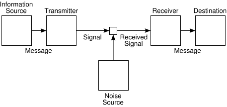
$\displaystyle \langle u \rangle = \sum_{i=1}^{n} p(x_i) u_i = - \sum_{i=1}^{n} p(x_i) \log_b (p(x_i))$

gray-level histogram -> probability density p(x_k) -> entropy

http://en.wikipedia.org/wiki/Entropy_(information_theory)

Shannon's source coding theorem shows that, in the limit, the average length of the shortest possible representation to encode the messages in a given alphabet is their entropy divided by the logarithm of the number of symbols in the target alphabet.

C.E. Shannon, "A Mathematical Theory of Communication",

shannon1948.pdf

Bell System Technical Journal, vol. 27, pp. 379-423, 623-656, July, October, 1948

2.3.4 Visual perception of the image

Contrast

http://en.wikipedia.org/wiki/Contrast_(vision)

Acuity 예민함

http://en.wikipedia.org/wiki/Visual_acuity

visual illusions

http://en.wikipedia.org/wiki/Optical_illusion

http://en.wikipedia.org/wiki/Ebbinghaus_illusion

perceptual grouping -> image segmentation

Gestalt theory

http://en.wikipedia.org/wiki/Gestalt_psychology

Patterns take precedence over elements and have properties that are not inherent in the elements themselves.

28p

2.3.5 Image quality

Azriel Rosenfeld, Avinash C. Kak, Digital Picture Processing, Academic Press, 1982

parameter optimization
correlation between images
resolution of small or proximate objects in the image
measures of image similarity (retrieval from image databases)

2.3.6 Noise in image

white noise
http://en.wikipedia.org/wiki/White_noise

-> Gaussian noise

additive noise
http://en.wikipedia.org/wiki/Additive_white_Gaussian_noise

multiplicative noise

quantization noise
http://en.wikipedia.org/wiki/Quantization_noise

impulse noise

-> salt-and-pepper noise
http://en.wikipedia.org/wiki/Salt_and_pepper_noise

unknown about noise properties -> local pre-processing methods
known noise parameters -> image restoration techniques

SNR = signal-to-noise ration
http://en.wikipedia.org/wiki/Signal-to-noise_ratio

2.4 Color images

2.4.1 Physics of color
2.4.2 Color perceived by humans
2.4.3 Color spaces
2.4.4 Palette images
2.4.5 Color constancy

2.5 Cameras: an overview

2.5.1 Photosensitive sensors
2.5.2 A monochromatic camera
2.5.3 A color camera

2.6 Summary

'@GSMC > 박래홍: Computer Vision' 카테고리의 다른 글

Ch.10 Image Understanding (0)	2008.12.15
Ch.9 Object Recognition (0)	2008.11.25
2.4 Color images & 2.5 Cameras (0)	2008.10.16
Ch. 6 Segmentation I (0)	2008.09.20
Ch.1 Introduction (0)	2008.09.04

posted by maetel

Ch.1 Introduction

2008. 9. 4. 21:49 @GSMC/박래홍: Computer Vision

Image Representation (4 levels):
objects/ a scene - (2-d projection, sampling/quantizing)-> digital image - (regions, edges, scale, interest points, texture, motion) -> image with features -> objects

Image Analysis - computer vision techniques
- low level
1) image acquisition (captaured/sensed, digitized)
2) preprocessing (noise suppression, enhancement of some object features - eg. edge extraction)
3) image segmentation (objects from the background)

> higher level
1) reducing the data quantity
2) knowledge about the image content - object size, shape, etc
3) expressed in symbolic form (http://en.wikipedia.org/wiki/Formal_language)
4) feedback from high-level to low-level

digital manipulation -> preprocessing -> segmentation -> recognition -> understanding

'@GSMC > 박래홍: Computer Vision' 카테고리의 다른 글

Ch.10 Image Understanding (0)	2008.12.15
Ch.9 Object Recognition (0)	2008.11.25
2.4 Color images & 2.5 Cameras (0)	2008.10.16
Ch. 6 Segmentation I (0)	2008.09.20
Ch. 2 The image, its representations and properties (0)	2008.09.10

posted by maetel

Pattern Classification: ch.1 Introduction

2008. 9. 3. 21:12 @GSMC/김경환: Pattern Recognition

Pattern Recognition
; the act of tacking in raw data and making an action based on the "category" of the pattern
- evolving highly sophisticated neural and cognitive systems

Machine Perception

http://en.wikipedia.org/wiki/Machine_perception
: the ability of computing machines to sense and interpret images, sounds, or other contents of their environments, or of the contents of stored media

http://en.wikipedia.org/wiki/Machine_vision
machine vision most often requires also digital input/output devices and computer networks to control other manufacturing equipment such as robotic arms. Machine Vision is a subfield of engineering that encompasses computer science, optics, mechanical engineering, and industrial automation.

machine vision systems use digital cameras, smart cameras and image processing software to perform similar inspections.
Machine vision systems are programmed to perform narrowly defined tasks such as counting objects on a conveyor, reading serial numbers, and searching for surface defects.

http://en.wikipedia.org/wiki/Speech_recognition

Pattern Recognition

http://en.wikipedia.org/wiki/Pattern_recognition
Pattern recognition is a sub-topic of machine learning. It can be defined as

"the act of taking in raw data and taking an action based on the category of the data".

Most research in pattern recognition is about methods for supervised learning and unsupervised learning.

Pattern recognition aims to classify data (patterns) based on either a priori knowledge or on statistical information extracted from the patterns. The patterns to be classified are usually groups of measurements or observations, defining points in an appropriate multidimensional space. This is in contrast to pattern matching, where the pattern is rigidly specified.

optical character recognition

http://en.wikipedia.org/wiki/Optical_character_recognition
the mechanical or electronic translation of images of handwritten, typewritten or printed text (usually captured by a scanner) into machine-editable text

pilot (adj) experimental

models - descriptions - mathematical in form (*분류할 대상의 종류들 classes 사이의 차이점을 수학적으로 기술한 것)

pattern classification

1) to hypothesize the class of the models

2) to process the sensed data to eliminate noise (not due to the models)

3) to choose the model that corresponds best for any sensed pattern

preprocessing - to simplify subsequent operations without losing relevant information

feature extraction - to reduce the data by measuring certain "features" or "properties"

classification - to evaluate the evidence presented and make a final decision

http://en.wikipedia.org/wiki/Information_flow

training sample (*feature로 가정한 변수(예. 길이)의 threshold를 설정하기 위하여 전체 입력 데이터 중에서 선택하여 변수에 대한 측정값을 얻는 데 사용하는 일부의 데이터)

http://en.wikipedia.org/wiki/Data

cost

'@GSMC > 김경환: Pattern Recognition' 카테고리의 다른 글

ch.6 Multilayer Neural Networks (0)	2008.11.21
ch.5 Linear Discriminant Functions (0)	2008.11.02
ch.4 Nonparametric Techniques (0)	2008.10.21
ch.3 Maximum-Likelihood and Bayesian Parameter Estimation (0)	2008.10.08
ch.2 Bayesian Decision Theory (0)	2008.09.25

posted by maetel

[심귀보] 유전자 알고리즘

2008. 7. 7. 18:17 @GSMC/정문열: Generative Art

중앙대학교 심귀보 Kwee-Bo Sim

http://alife.cau.ac.kr/korean/sub01/GAs.html

'@GSMC > 정문열: Generative Art' 카테고리의 다른 글

breadth-first search (0)	2008.06.30
Evolutionary and Swarm Design (0)	2008.06.27
genetic programming (0)	2008.06.05
treemaps (0)	2008.05.29
변수 (0)	2008.05.17

posted by maetel

breadth-first search

2008. 6. 30. 03:38 @GSMC/정문열: Generative Art

ref.

http://en.wikipedia.org/wiki/Breadth-first_search
(5번 숙제 관련)

http://en.wikipedia.org/wiki/Depth-first_search
(4번 숙제 관련)

http://en.wikipedia.org/wiki/Tree_traversal

'@GSMC > 정문열: Generative Art' 카테고리의 다른 글

[심귀보] 유전자 알고리즘 (0)	2008.07.07
Evolutionary and Swarm Design (0)	2008.06.27
genetic programming (0)	2008.06.05
treemaps (0)	2008.05.29
변수 (0)	2008.05.17

posted by maetel

Evolutionary and Swarm Design

2008. 6. 27. 17:45 @GSMC/정문열: Generative Art

Evolutionary and Swarm Design
CPSC 599.33 — Summer 2001
Christian Jacob — jacob@cpsc.ucalgary.ca
http://www.cpsc.ucalgary.ca/~jacob
03 July 2001

invalid-file

Penousal Machado : Neural Evolutionary Art
http://eden.dei.uc.pt/~machado/

Ken Musgrave: Genetic Programming and Genetic Art
www.wizardnet.com/musgrave/mutatis.html
www.fractalworlds.com

Steven Rooke: Evolutionary Art

Jano van Hemert: Art by Evolution on the Web
http://www.vanhemert.co.uk/

Piet Mondriaan — Theo van Doesburg — Mandala art — Fractal art

Jeffrey Ventrella: Art and Artificial Life
www.ventrella.com

Mattias Fagerlund: Cambrian Art
http://www.hypeskeptic.com/mattias/

The NeuroEvolution of Augmenting Topologies (NEAT)
http://www.cs.ucf.edu/~kstanley/neat.html

Andrej Bauer: Random Art (Carnegie Mellon University)
http://andrej.com/

Aaron — The Robot as an Artist
http://www.aaai.org/AITopics/pmwiki/pmwiki.php/AITopics/Art#aaron

Evolutionary Computer Graphics

http://www.artlandia.com/
Igor Bakshee

http://www.graphica.com/
Michael Trott

Organic Genetic and Evolutionary Art

Andrew Rowbottom
http://www.netlink.co.uk/~snaffle/form/evolutio.html

Evolutionary Art and Computers
Stephen Todd
William Latham

Organic Art
William Latham
http://www.doc.gold.ac.uk/~mas01whl/

Mark Atkinson

Linda Moss

Genetic L-System Programming

Swarm Systems
· Cell Replication
· Competitive Cell Replication
· "BlocksWorld"

Design by Swarms

Turtle Art
Example projects by Namrata Khemka

Self-Assembly

Swarm Art by Euan Forrester

'@GSMC > 정문열: Generative Art' 카테고리의 다른 글

[심귀보] 유전자 알고리즘 (0)	2008.07.07
breadth-first search (0)	2008.06.30
genetic programming (0)	2008.06.05
treemaps (0)	2008.05.29
변수 (0)	2008.05.17

posted by maetel

class 13 - mapping: bump + specular

2008. 6. 20. 15:15 @GSMC/정재환: 3D Modeling&Rendering

2008-06-20 쇠 @가브리엘 504

기본 매핑

color + bump + speacular

'@GSMC > 정재환: 3D Modeling&Rendering' 카테고리의 다른 글

class 12 (0)	2008.06.13
class 10 - mapping (0)	2008.05.30
class 9 공룡 만들기 (0)	2008.05.23
class 7 - 돌고래 완성 (0)	2008.05.02
class 6 - dolphin (0)	2008.04.25

posted by maetel

class 12

2008. 6. 13. 17:08 @GSMC/정재환: 3D Modeling&Rendering

rendering 모드
(1)
window>render edits> render settings

targa
tiff (추천)

image size: a4
resolution: 300 dpi

maya software

quality: production quality

raytracing quality: raytracing 체크

(2)
render
batch render

'@GSMC > 정재환: 3D Modeling&Rendering' 카테고리의 다른 글

class 13 - mapping: bump + specular (0)	2008.06.20
class 10 - mapping (0)	2008.05.30
class 9 공룡 만들기 (0)	2008.05.23
class 7 - 돌고래 완성 (0)	2008.05.02
class 6 - dolphin (0)	2008.04.25

posted by maetel

[Steve Oualline] 13. Simple Pointers

2008. 6. 10. 20:26 @GSMC/서용덕: DMD Programming

Steve Oualline
Practical C Programming

13. Simple Pointers

183p
Pointers are also called address variables because they contain the addresses of other variables.

184p
Pointers can be used as a quick and simple way to access arrays. (...) Pointers can be used to create new variables and complex data structures such as linked lists and trees.

185p
The operator ampersand (&) returns the address of a thing which is a pointer.
The operator asterisk (*) returns the object to which a pointer points.

Operator - Meaning
* - Dereference (given a pointer, get the thing referenced)
& - Address of (given a thing, point to it)

The operator ampersand (&) returns the address of a thing which is a pointer.
The operator asterisk (*) returns the object to which a pointer points.

int *thing_ptr; // declare a pointer to a thing
thing_ptr = &thing; // point to the thing
*thing_ptr = 5; // set "thing" to 5
// The expression &thing is a pointer to a thing. The variable thing is an object
// thing_ptr points to any integer. It may or may not point to the specific variable thing.

The & (address of operator) gets the address of an object (a pointer).
The * (dereference operator) tells C to look at the data pointed to, not hte pointer itself.

http://www.cplusplus.com/doc/tutorial/pointers.html

http://www.cprogramming.com/tutorial/lesson6.html

187p
Several pointers can point to the same thing.

188p
Pointers as Function Arguments

The only result of a function is a single return value.

http://en.wikipedia.org/wiki/Call_by_value#Call_by_value

http://www.cplusplus.com/doc/tutorial/functions2.html

NULL pointer
locale.h
http://www.cplusplus.com/reference/clibrary/clocale/

189p
const Pointers

const char *answer_ptr = "Forty-Two";

char *const name_ptr = "Test";

const char *const title_ptr = "Title";

191p
Pointers and Arrays

(reminding...) 서 교수님:
number[10] 이라고 배열 선언을 하면 컴파일러는 10개의 연속된 데이터를 위한 공간을 확보하고 그 첫번째 공간의 주소를 number 에 넣습니다. 그래서 number 는 number[0] 의 주소를 가지는 것입니다.

number[1] 은 배열에서 number[0] 다음의 값을 가지는데 그 공간의 주소값을 알고 싶으면 &number[1] 이라고 하든지 number+1 이라고 하면 됩니다.

거꾸로, number 에서 시작하여 두번째 즉 number[1] 의 값을 주소로부터 얻고 싶으면 number[1] 이라고 하든지 *(number+1) 로 하여 얻을 수 있습니다.

192p
A pointer can be used to find each element of the array.

197p
Using Pointers to Split a String

strchr()
http://www.cplusplus.com/reference/clibrary/cstring/strchr.html

201p
Pointers and Structures

Instead of having to move a lot of data around, we can declare an array of pointers and then sort the pointers.

Command-Line Arguments

main (int argc, char *argv[])
{

The parameter argc is the number of arguments on the command line (including the program name).
The array argv contains the actual arguments.

(reminding...)
터미널에서, 말씀하신대로 "./V2008122-01 input.txt"라고 치면 다음과 같이 나옵니다.
argc=2
argv[0]=./V2008122-01
argv[1]=input.txt

서 교수님:
argv[0] = 실행프로그램 이름; 1번째는 항상 실행프로그램의 패스/이름 이 들어갑니다.
이번에는 argv[1] 에 들어갈 두 번째 값을 주었기 때문에 그 값이 프린트 된 것입니다.
command-line arguments는 shell 프로그램이 fileio 함수를 호출할 때 매개변수로 주는 것이고, 좀 더 엄밀하게는 OS 가 main 함수를 호출할 때 주는 것입니다.

http://www.cplusplus.com/reference/clibrary/cstdio/fprintf.html

Example 13-12: print.c

// formats files for printing
// usage: print [options] file(s)

#include <stdio.h>
#include <stdlib.h>

int verbose = 0; // verbose mode (default = false)
char *out_file = "print.out"; //output filename
char *program_name; // name of the program for erros
int line_max = 66; // number of lines per page

void do_file(char *name)
{
printf("Verbose %d Lines %d Input %s Output %s\n",
   verbose, line_max, name, out_file);
}

void usage (void)
{
fprintf(stderr, "Usage is %s [options] [file-list]\n",
program_name);
fprintf(stderr, "Options\n");
fprintf(stderr, "    -v    verbose\n");
fprintf(stderr, "    -l<number> Number of line\n");
fprintf(stderr, "    -o<name>    Set output filename\n");
exit(8);
}

int main (int argc, char *argv[])
{
program_name =argv[0];

while ( (argc>1) && (argv[1][0] == '-') )
// argv[1][1] is the actual option character
{
switch (argv[1][1]) {
case 'v':
verbose = 1;
break;

case 'o':
out_file = &argv[1][2];
break;

case 'l':
line_max = atoi(&argv[1][2]);
break;

default:
fprintf(stderr, "Bad option %s\n", argv[1]);
usage();
}

++argv;
--argc;
}

if (argc == 1) {
do_file("printf.in");
}
else {
while (argc>1)
{
do_file(argv[1]);
++argv;
--argc;
}
}

return(0);
}

Xcode 실행창:

Verbose 0 Lines 66 Input printf.in Output print.out

terminal:

999:~/cintro/ch13/eg12 lym$ ./ch13eg12
Verbose 0 Lines 66 Input printf.in Output print.out
999:~/cintro/ch13/eg12 lym$ ./ch13eg12 i am tired
Verbose 0 Lines 66 Input i Output print.out
Verbose 0 Lines 66 Input am Output print.out
Verbose 0 Lines 66 Input tired Output print.out
999:~/cintro/ch13/eg12 lym$ ./ch13eg12 -v -l128 -0title xfile yfile zfile
Bad option -0title
Usage is ./ch13eg12 [options] [file-list]
Options
-v verbose
-l<number> Number of line
-o<name> Set output filename
999:~/cintro/ch13/eg12 lym$ ./ch13eg12 -v -l128 -otitle xfile yfile zfile
Verbose 1 Lines 128 Input xfile Output title
Verbose 1 Lines 128 Input yfile Output title
Verbose 1 Lines 128 Input zfile Output title

208p
A pointer does not create any new space for data, but just refers to data that is created elsewhere.

http://www.cplusplus.com/doc/tutorial/pointers.html
The identifier of an array is equivalent to the address of its first element, as a pointer is equivalent to the address of the first element that it points to, so in fact they are the same concept.

An array can be considered a constant pointer.

http://www.cprogramming.com/tutorial/lesson6.html
Arrays can act just like pointers.

'@GSMC > 서용덕: DMD Programming' 카테고리의 다른 글

Similarity Transformation (0)	2008.06.10
hw 9 - ppm 이미지 회전시키기 (0)	2008.05.30
[Steve Oualline] 12. Advanced Types (0)	2008.05.28
data type 정리 (0)	2008.05.24
[Steve Oualline] 11. Bit Operations (0)	2008.05.14

posted by maetel

Similarity Transformation

2008. 6. 10. 20:25 @GSMC/서용덕: DMD Programming

similarity transformation

http://mathworld.wolfram.com/SimilarityTransformation.html

invalid-file

'@GSMC > 서용덕: DMD Programming' 카테고리의 다른 글

[Steve Oualline] 13. Simple Pointers (0)	2008.06.10
hw 9 - ppm 이미지 회전시키기 (0)	2008.05.30
[Steve Oualline] 12. Advanced Types (0)	2008.05.28
data type 정리 (0)	2008.05.24
[Steve Oualline] 11. Bit Operations (0)	2008.05.14

posted by maetel

genetic programming

2008. 6. 5. 09:45 @GSMC/정문열: Generative Art

evaluating fitness
http://en.wikipedia.org/wiki/Fitness_function

cross-over
mutation

http://en.wikipedia.org/wiki/Roulette_wheel_selection

'@GSMC > 정문열: Generative Art' 카테고리의 다른 글

breadth-first search (0)	2008.06.30
Evolutionary and Swarm Design (0)	2008.06.27
treemaps (0)	2008.05.29
변수 (0)	2008.05.17
class 5/1 (0)	2008.05.01

posted by maetel

Search

Tag

Notice

Recent Post

Recent Comment

Recent Trackback

Archive

My Link

calendar

Category

'@GSMC'에 해당되는 글 122건

'@GSMC > 김경환: Pattern Recognition' 카테고리의 다른 글

'@GSMC > 김경환: Pattern Recognition' 카테고리의 다른 글

'@GSMC > 이상욱: Principles of Human and Artificial Vision' 카테고리의 다른 글

'@GSMC > 이상욱: Principles of Human and Artificial Vision' 카테고리의 다른 글

'@GSMC > 이상욱: Principles of Human and Artificial Vision' 카테고리의 다른 글

'@GSMC > 이상욱: Principles of Human and Artificial Vision' 카테고리의 다른 글

'@GSMC > 이상욱: Principles of Human and Artificial Vision' 카테고리의 다른 글

'@GSMC > 이상욱: Principles of Human and Artificial Vision' 카테고리의 다른 글

'@GSMC > 이상욱: Principles of Human and Artificial Vision' 카테고리의 다른 글

'@GSMC > 김경환: Pattern Recognition' 카테고리의 다른 글

'@GSMC > 박래홍: Computer Vision' 카테고리의 다른 글

'@GSMC > 김경환: Pattern Recognition' 카테고리의 다른 글

'@GSMC > 김경환: Pattern Recognition' 카테고리의 다른 글

'@GSMC > 박래홍: Computer Vision' 카테고리의 다른 글

'@GSMC > 박래홍: Computer Vision' 카테고리의 다른 글

'@GSMC > 박래홍: Computer Vision' 카테고리의 다른 글

'@GSMC > 김경환: Pattern Recognition' 카테고리의 다른 글

'@GSMC > 정문열: Generative Art' 카테고리의 다른 글

'@GSMC > 정문열: Generative Art' 카테고리의 다른 글

'@GSMC > 정문열: Generative Art' 카테고리의 다른 글

'@GSMC > 정재환: 3D Modeling&Rendering' 카테고리의 다른 글

'@GSMC > 정재환: 3D Modeling&Rendering' 카테고리의 다른 글

'@GSMC > 서용덕: DMD Programming' 카테고리의 다른 글

'@GSMC > 서용덕: DMD Programming' 카테고리의 다른 글

'@GSMC > 정문열: Generative Art' 카테고리의 다른 글

티스토리툴바