블로그 이미지
Leeway is... the freedom that someone has to take the action they want to or to change their plans.
maetel

Notice

Recent Post

Recent Comment

Recent Trackback

Archive

calendar

1 2 3 4 5 6
7 8 9 10 11 12 13
14 15 16 17 18 19 20
21 22 23 24 25 26 27
28 29 30
  • total
  • today
  • yesterday

Category

2010. 3. 24. 20:23 Footmarks
서강대학교 영상대학원 기업 특강: 3D 영상산업의 전망과 동향
강사: Stereo Pictures 성필문 회장

2010-03-24 수 늦은 5시 @가브리엘관 704호


Introduction: 영상 산업의 Reality 향상에 대한 노력

변화의 시작:
Hollywood 영화감독들
미국 영화 관객
Digital 3D 영화관
과거의 Analog 3D movies
최근의 Digital 3D movies
Digital 3D TV

입체영상의 제작 방법

입체영상 제작의 대안: 2D to 3D converting

Hollywood의 움직임

입체영상 컨텐츠 산업의 전망


스테레오픽처스
http://stereopictures.com/
 
Sasson Film Design (Canada)
http://www.sassoonfilmdesign.com/

Convergence ---


posted by maetel
2010. 3. 15. 15:56 Computer Vision
Three-dimensional computer vision: a geometric viewpoint 
By Olivier Faugeras

googleBooks
mitpress

'Computer Vision' 카테고리의 다른 글

Canny edge detection  (0) 2010.03.30
ARToolKit - simpleTest  (0) 2010.03.17
opencv: video capturing from a camera  (4) 2010.03.13
Leordeanu & Hebert, "Unsupervised learning for graph matching"  (0) 2010.03.04
ARToolKit test log  (0) 2010.03.03
posted by maetel
2010. 2. 22. 19:25 Computer Vision
UX, interactive art 분야 조사

1
Buzz 3D 사의 - 3D Interface - High Definition digital 3D Marketing solution
http://www.buzz3d.com/3d_interface_index.html
: 웹에서 실시간으로 동작 가능한 3차원 가상 현실 구현 플랫폼/애플리케이션
-> 사용자 트래킹: http://www.buzz3d.com/3d_interface_features_user.html
을 통해 행동을 분석하고
-> 햅틱: http://www.buzz3d.com/3d_interface_features_haptics.html
기능을 통해 체감형 경험을 제공함


2
HTC 사의 휴대폰 - HTC Touch Diamond
-> TouchFLO 3D 기능: http://www.htc.com/www/product/touchdiamond/touchflo-3d.html
: finger gesture를 통해 메뉴 선택, 웹 브라우징, 이메일링 등을 할 수 있음


3
CityWall
http://citywall.org/
: 핀란드 헬싱키 중심에 설치되어 있는 대형 멀티 터치 디스플레이
Helsinki Institute for Information TechnologyMultitouch 사에서 공동 개발
http://www.youtube.com/watch?v=WkNq3cYGTPE


4
Microsoft 사의 Bing Maps의 augmented reality mapping 기술
: 사용자가 찍고 있는 동영상의 2차원 이미지를 웹 상의 3차원 지도와 실시간으로 매칭시켜 보여 줌 (이때 시간 정보까지 반영함으로써 4D를 실현)
http://www.ted.com/talks/blaise_aguera.html


5
3차원 UX 구현 툴 목록 (입력이 3차원이 아니므로 주제와 별개일 수도 있음)
http://www.artefactgroup.com/blog/2010/02/tools-for-building-a-3d-ux/
- PapervisionAway 3d 는 Adobe Flash의 plug-in들
- Electric Rain 사가 개발한 Swift 3d
- Scaleform 사의 게임 개발용 솔루션 GFx 3.0
- Microsoft 사의 Expression Blend
- Electric Rain 사의 3D XAML 툴 ZAM 3D
- 비프로그래머들을 위한 Processing으로 만들어진 ATOMIC Authoring Tool은 ARToolkit 라이브러리로 제공되는 증강 현실 저작 툴
- TAT kaster UI 렌더링 플랫폼
- Kanzi


6
R.U.S.E. : 손가락 동작을 통해 조작하는 게임으로 E3에 발표됐음
ref. http://www.artefactgroup.com/blog/2009/09/3d-ui-useful-usable-or-desirable/

7
SKT의 증강 현실 서비스 Ovjet
http://ovjet.com/
: 휴대폰 카메라로 보는 실제화면 위에 실시간으로 다양한 정보를 결합하여 보여주는 증강현실(Augmented Reality) 서비스
ref. http://news.cnbnews.com/category/read.html?bcode=102993


8
CATIA
제품디자인 제작을 위한 가상현실 저작 툴


9
Marisil (Mobile Augmented Reality Interface Sign Interpretation Language)
http://marisil.org/
손동작에 기반한 증강 현실을 인터페이스로하는 모바일 기술


10
http://www.engadget.com/2005/10/02/pioneer-develops-input-device-for-3d-drawing/


http://en.wikipedia.org/wiki/Gesture_recognition

http://en.wikipedia.org/wiki/Depth_perception

"human detection IP"
http://www.visionbib.com/bibliography/motion-f733.html
VideoProtein  http://www.videoprotein.com/

"depth map IP application"
http://altruisticrobot.tistory.com/219
posted by maetel
2009. 11. 10. 15:14 Computer Vision
1차원 particle filter 간단 예제
// 1-D Particle filter algorithm exercise
// 2009-11-06
// ref. Probabilistic Robotics: 98p

#include <iostream>
#include <cstdlib> //defining RAND_MAX
#include <ctime> //time as a random seed
#include <cmath>
using namespace std;

#define PI 3.14159265
#define N 10 //number of particles

////////////////////////////////////////////////////////////////////////////
// random number generators written by kyu
double uniform_random(void) {
   
    return (double) rand() / (double) RAND_MAX;
   
}

double gaussian_random(void) {
   
    static int next_gaussian = 0;
    static double saved_gaussian_value;
   
    double fac, rsq, v1, v2;
   
    if(next_gaussian == 0) {
       
        do {
            v1 = 2.0 * uniform_random() - 1.0;
            v2 = 2.0 * uniform_random() - 1.0;
            rsq = v1 * v1 + v2 * v2;
        }
        while(rsq >= 1.0 || rsq == 0.0);
        fac = sqrt(-2.0 * log(rsq) / rsq);
        saved_gaussian_value = v1 * fac;
        next_gaussian = 1;
        return v2 * fac;
    }
    else {
        next_gaussian = 0;
        return saved_gaussian_value;
    }
}

double normal_distribution(double mean, double standardDeviation, double state) {
   
    double variance = standardDeviation * standardDeviation;
   
    return exp(-0.5 * (state - mean) * (state - mean) / variance ) / sqrt(2 * PI * variance);
}

////////////////////////////////////////////////////////////////////////////


int main (int argc, char * const argv[]) {
   
    double groundtruth[] = {0.5, 2.0, 3.5, 5.0, 7.0, 8.0, 10.0};
    double measurement[] = {0.4, 2.1, 3.2, 5.3, 7.4, 8.1, 9.6};
    double transition_noise = 0.3; // covariance of Gaussian noise to control
    double measurement_noise = 0.3; // covariance of Gaussian noise to measurement
   
    double x[N]; // N particles
    double x_p[N]; // predicted particles
    double state; // estimated state with particles
    double x_u[N]; // temporary variables for updating particles
    double v[N]; // velocity
    double v_u[N]; // temporary variables for updating velocity   
    double m[N]; // measurement
    double l[N]; // likelihood
    double lsum; // sum of likelihoods
    double w[N]; // weight of each particle
    double a[N]; // portion between particles
   
    double grn[N]; // Gaussian random number
    double urn[N]; // uniform random number
   
    srand(time(NULL));        
   
    // initialize particles
    for (int n = 0; n < N; n++)
    {
        x[n] = 0.0;
        v[n] = 0.0;
        w[n] = (double)1/(double)N;           
    }
   
    int step = 7;
    for (int t = 0; t < step; t++)
    {
        cout << "step " << t << endl;       
        // measure
        m[t] = measurement[t];
       
        cout << "groundtruth = " << groundtruth[t] << endl;
        cout << "measurement = " << measurement[t] << endl;       
       
        lsum = 0;
        for (int n = 0; n < N; n++)
        {
            // predict
            grn[n] = gaussian_random();
            x_p[n] = x[n] + v[n] + transition_noise * grn[n];
//            cout << grn[n] << endl;
           
            // estimate likelihood between measurement and each prediction
            l[n] = normal_distribution(m[t], measurement_noise, x_p[n]); // ref. 14p eqn(2.3)
            lsum += l[n];
        }
//            cout << "lsum = " << lsum << endl;       
       
        // estimate states       
        state = 0;
        for (int n = 0; n < N; n++)
        {
            w[n] = l[n] / lsum; // update normalized weights of particles           
//            cout << "w" << n << "= " << w[n] << "  ";               
            state += w[n] * x_p[n]; // estimate the state with particles
        }   
        cout << "estimation = " << state << endl;
       
        // update       
        // define integrated portions of each particles; 0 < a[0] < a[1] < a[2] = 1
        a[0] = w[0];
        for (int n = 1; n < N; n++)
        {
            a[n] = a[n - 1] + w[n];
//            cout << "a" << n << "= " << a[n] << "  ";           
        }
        for (int n = 0; n < N; n++)
        {   
            // select a particle from the distribution
            urn[n] = uniform_random();
            int select;
            for (int k = 0; k < N; k++)
            {
                if (urn[n] < a[k] )
                {
                    select = k;
                    break;
                }
            }
            cout << "select" << n << "= " << select << "  ";       
            // retain the selection 
            x_u[n] = x_p[select];
            v_u[n] = x_p[select] - x[select];
        }
        cout << endl << endl;
        // updated each particle and its velocity
        for (int n = 0; n < N; n++)
        {
            x[n] = x_u[n];
            v[n] = v_u[n];
//            cout << "v" << n << "= " << v[n] << "  ";   
        }
    }
   
    return 0;
}


실행 결과:


2차원 particle filter 간단 예제

// 2-D Particle filter algorithm exercise
// 2009-11-10
// ref. Probabilistic Robotics: 98p

#include <OpenCV/OpenCV.h> // matrix operations
#include <iostream>
#include <cstdlib> // RAND_MAX
#include <ctime> // time as a random seed
#include <cmath>
#include <algorithm>
using namespace std;

#define PI 3.14159265
#define N 100 //number of particles

// uniform random number generator
double uniform_random(void) {
   
    return (double) rand() / (double) RAND_MAX;
   
}

// Gaussian random number generator
double gaussian_random(void) {
   
    static int next_gaussian = 0;
    static double saved_gaussian_value;
   
    double fac, rsq, v1, v2;
   
    if(next_gaussian == 0) {
       
        do {
            v1 = 2.0 * uniform_random() - 1.0;
            v2 = 2.0 * uniform_random() - 1.0;
            rsq = v1 * v1 + v2 * v2;
        }
        while(rsq >= 1.0 || rsq == 0.0);
        fac = sqrt(-2.0 * log(rsq) / rsq);
        saved_gaussian_value = v1 * fac;
        next_gaussian = 1;
        return v2 * fac;
    }
    else {
        next_gaussian = 0;
        return saved_gaussian_value;
    }
}

double normal_distribution(double mean, double standardDeviation, double state) {
   
    double variance = standardDeviation * standardDeviation;
   
    return exp(-0.5 * (state - mean) * (state - mean) / variance ) / sqrt(2 * PI * variance);
}
////////////////////////////////////////////////////////////////////////////

// set groundtruth
void set_groundtruth (CvMat* groundtruth, double x, double y)
{
    cvmSet(groundtruth, 0, 0, x); // x-value
    cvmSet(groundtruth, 1, 0, y); // y-value
   
    cout << "groundtruth = " << cvmGet(groundtruth,0,0) << "  " << cvmGet(groundtruth,1,0) << endl;
}


// count the number of detections in measurement process
int count_detections (void)
{
    // set cases of measurement results
    double mtype[4];
    mtype [0] = 0.0;
    mtype [1] = 0.5;
    mtype [2] = mtype[1] + 0.3;
    mtype [3] = mtype[2] + 0.2;
//    cout << "check measurement type3 = " << mtype[3] << endl; // just to check

    // select a measurement case
    double mrn = uniform_random();       
    int type = 1;
    for ( int k = 0; k < 3; k++ )
    {   
        if ( mrn < mtype[k] )
        {
            type = k;
            break;
        }
    }
    return type;
}

// distance between measurement and prediction
double distance(CvMat* measurement, CvMat* prediction)
{
    double distance2 = 0;
    double differance = 0;
    for (int u = 0; u < 2; u++)
    {
        differance = cvmGet(measurement,u,0) - cvmGet(prediction,u,0);
        distance2 += differance * differance;
    }
    return sqrt(distance2);
}


// likelihood based on multivariative normal distribution (ref. 15p eqn(2.4))
double likelihood(CvMat *mean, CvMat *covariance, CvMat *sample) {
   
    CvMat* diff = cvCreateMat(2, 1, CV_64FC1);
    cvSub(sample, mean, diff); // sample - mean -> diff
    CvMat* diff_t = cvCreateMat(1, 2, CV_64FC1);
    cvTranspose(diff, diff_t); // transpose(diff) -> diff_t
    CvMat* cov_inv = cvCreateMat(2, 2, CV_64FC1);
    cvInvert(covariance, cov_inv); // transpose(covariance) -> cov_inv
    CvMat* tmp = cvCreateMat(2, 1, CV_64FC1);
    CvMat* dist = cvCreateMat(1, 1, CV_64FC1);
    cvMatMul(cov_inv, diff, tmp); // cov_inv * diff -> tmp   
    cvMatMul(diff_t, tmp, dist); // diff_t * tmp -> dist
   
    double likeliness = exp( -0.5 * cvmGet(dist, 0, 0) );
    double bound = 0.0000001;
    if ( likeliness < bound )
    {
        likeliness = bound;
    }
    return likeliness;
//    return exp( -0.5 * cvmGet(dist, 0, 0) );
//    return max(0.0000001, exp(-0.5 * cvmGet(dist, 0, 0)));   
   
}


/*
struct particle
{
    double weight; // weight of a particle
    CvMat* loc_p = cvCreateMat(2, 1, CV_64FC1); // previously estimated position of a particle
    CvMat* loc = cvCreateMat(2, 1, CV_64FC1); // currently estimated position of a particle
    CvMat* velocity = cvCreateMat(2, 1, CV_64FC1); // estimated velocity of a particle
    cvSub(loc, loc_p, velocity); // loc - loc_p -> velocity
};
*/


int main (int argc, char * const argv[]) {
   
    srand(time(NULL));

    int width = 400; // width of image window
    int height = 400; // height of image window   
   
    IplImage *iplImg = cvCreateImage(cvSize(width, height), 8, 3);
    cvZero(iplImg);
   
    cvNamedWindow("ParticleFilter-2d", 0);
   
   
     // covariance of Gaussian noise to control
    CvMat* transition_noise = cvCreateMat(2, 2, CV_64FC1);
    cvmSet(transition_noise, 0, 0, 3); //set transition_noise(0,0) to 0.1
    cvmSet(transition_noise, 0, 1, 0.0);
    cvmSet(transition_noise, 1, 0, 0.0);
    cvmSet(transition_noise, 1, 1, 6);      
   
    // covariance of Gaussian noise to measurement
    CvMat* measurement_noise = cvCreateMat(2, 2, CV_64FC1);
    cvmSet(measurement_noise, 0, 0, 2); //set measurement_noise(0,0) to 0.3
    cvmSet(measurement_noise, 0, 1, 0.0);
    cvmSet(measurement_noise, 1, 0, 0.0);
    cvmSet(measurement_noise, 1, 1, 2);  
   
    CvMat* state = cvCreateMat(2, 1, CV_64FC1);
    // declare particles
/*    particle pb[N]; // N estimated particles
    particle pp[N]; // N predicted particles       
    particle pu[N]; // temporary variables for updating particles       
*/
    CvMat* pb [N]; // estimated particles
    CvMat* pp [N]; // predicted particles
    CvMat* pu [N]; // temporary variables to update a particle
    CvMat* v[N]; // estimated velocity of each particle
    CvMat* vu[N]; // temporary varialbe to update the velocity   
    double w[N]; // weight of each particle
    for (int n = 0; n < N; n++)
    {
        pb[n] = cvCreateMat(2, 1, CV_64FC1);
        pp[n] = cvCreateMat(2, 1, CV_64FC1);
        pu[n] = cvCreateMat(2, 1, CV_64FC1);   
        v[n] = cvCreateMat(2, 1, CV_64FC1);   
        vu[n] = cvCreateMat(2, 1, CV_64FC1);           
    }   
   
    // initialize particles and the state
    for (int n = 0; n < N; n++)
    {
        w[n] = (double) 1 / (double) N; // equally weighted
        for (int row=0; row < 2; row++)
        {
            cvmSet(pb[n], row, 0, 0.0);
            cvmSet(v[n], row, 0, 15 * uniform_random());
            cvmSet(state, row, 0, 0.0);           
        }
    }
   
    // set the system   
    CvMat* groundtruth = cvCreateMat(2, 1, CV_64FC1); // groundtruth of states   
    CvMat* measurement [3]; // measurement of states
    for (int k = 0; k < 3; k++) // 3 types of measurement
    {
        measurement[k] = cvCreateMat(2, 1, CV_64FC1);
    }
   
    cout << "start filtering... " << endl << endl;
    int step = 30; //30; // timestep
   
    for (int t = 0; t < step; t++) // for "step" steps
    {
//        cvZero(iplImg);
        cout << "step " << t << endl;
       
        // set groundtruth
        double gx = 10 * t;
        double gy = (-1.0 / width ) * (gx - width) * (gx - width) + height;
        set_groundtruth(groundtruth, gx, gy);

        // set measurement types
        double c1 = 1.0, c2 = 4.0;   
        // measured point 1
        cvmSet(measurement[0], 0, 0, gx + (c1 * cvmGet(measurement_noise,0,0) * gaussian_random())); // x-value
        cvmSet(measurement[0], 1, 0, gy + (c1 * cvmGet(measurement_noise,1,1) * gaussian_random())); // y-value
        // measured point 2
        cvmSet(measurement[1], 0, 0, gx + (c2 * cvmGet(measurement_noise,0,0) * gaussian_random())); // x-value
        cvmSet(measurement[1], 1, 0, gy + (c2 * cvmGet(measurement_noise,1,1) * gaussian_random())); // y-value
        // measured point 3 // clutter noise
        cvmSet(measurement[2], 0, 0, width*uniform_random()); // x-value
        cvmSet(measurement[2], 1, 0, height*uniform_random()); // y-value       

        // count the number of measurements       
        int count = count_detections(); // number of detections
        cout << "# of measured points = " << count << endl;
   
        // get measurement           
        for (int index = 0; index < count; index++)
        {
            cout << "measurement #" << index << " : "
                << cvmGet(measurement[index],0,0) << "  " << cvmGet(measurement[index],1,0) << endl;
           
            cvCircle(iplImg, cvPoint(cvRound(cvmGet(measurement[index],0,0)), cvRound(cvmGet(measurement[index],1,0))), 4, CV_RGB(200, 0, 255), 1);
           
        }
       
       
        double like[N]; // likelihood between measurement and prediction
        double like_sum = 0; // sum of likelihoods
       
        for (int n = 0; n < N; n++) // for "N" particles
        {
            // predict
            double prediction;
            for (int row = 0; row < 2; row++)
            {
               
                prediction = cvmGet(pb[n],row,0) + cvmGet(v[n],row,0) + cvmGet(transition_noise,row,row) * gaussian_random();
                cvmSet(pp[n], row, 0, prediction);
            }
           
            cvLine(iplImg, cvPoint(cvRound(cvmGet(pp[n],0,0)), cvRound(cvmGet(pp[n],1,0))), cvPoint(cvRound(cvmGet(pb[n],0,0)), cvRound(cvmGet(pb[n],1,0))), CV_RGB(100,100,0), 1);           
            cvCircle(iplImg, cvPoint(cvRound(cvmGet(pp[n],0,0)), cvRound(cvmGet(pp[n],1,0))), 1, CV_RGB(255, 255, 0));


            // evaluate measurements
            double range = (double) width; // range to search measurements for each particle
//            cout << "range of distances = " << range << endl;
            int mselected;
            for (int index = 0; index < count; index++)
            {
                double d = distance(measurement[index], pp[n]);
               
                if ( d < range )
                {
                    range = d;
                    mselected = index; // selected measurement
                }
            }
///            cout << "selected measurement # = " << mselected << endl;
            like[n] = likelihood(measurement[mselected], measurement_noise, pp[n]);   
       
///            cout << "likelihood of #" << n << " = " << like[n] << endl;
           
            like_sum += like[n];
        }
       
///        cout << "sum of likelihoods = " << like_sum << endl;
       
        // estimate states       
        double state_x = 0.0;
        double state_y = 0.0;
   
        // estimate the state with predicted particles
        for (int n = 0; n < N; n++) // for "N" particles
        {
            w[n] = like[n] / like_sum; // update normalized weights of particles           
///            cout << "w" << n << "= " << w[n] << "  ";               
            state_x += w[n] * cvmGet(pp[n], 0, 0); // x-value
            state_y += w[n] * cvmGet(pp[n], 1, 0); // y-value
        }
        cvmSet(state, 0, 0, state_x);
        cvmSet(state, 1, 0, state_y);       
       
        cout << endl << "* * * * * *" << endl;       
        cout << "estimation = " << cvmGet(state,0,0) << "  " << cvmGet(state,1,0) << endl;
        cvCircle(iplImg, cvPoint(cvRound(cvmGet(state,0,0)), cvRound(cvmGet(state,1,0))), 4, CV_RGB(0, 255, 200), 2);
   
        // update particles       
        cout << endl << "updating particles" << endl;
        double urn[N]; // uniform random number
        double a[N]; // portion between particles

        // define integrated portions of each particles; 0 < a[0] < a[1] < a[2] = 1
        a[0] = w[0];
        for (int n = 1; n < N; n++)
        {
            a[n] = a[n - 1] + w[n];
//            cout << "a" << n << "= " << a[n] << "  ";           
        }
//        cout << "a" << N << "= " << a[N] << "  " << endl;           
       
        for (int n = 0; n < N; n++)
        {   
            // select a particle from the distribution
            urn[n] = uniform_random();
            int pselected;
            for (int k = 0; k < N; k++)
            {
                if (urn[n] < a[k] )
                {
                    pselected = k;
                    break;
                }
            }
///            cout << "particle " << n << " => " << pselected << "  ";       
            // retain the selection 
            cvmSet(pu[n], 0, 0, cvmGet(pp[pselected],0,0)); // x-value
            cvmSet(pu[n], 1, 0, cvmGet(pp[pselected],1,0)); // y-value
           
            cvSub(pp[pselected], pb[pselected], vu[n]); // pp - pb -> vu
   
        }
        // updated each particle and its velocity
        for (int n = 0; n < N; n++)
        {
            for (int row = 0; row < 2; row++)
            {
                cvmSet(pb[n], row, 0, cvmGet(pu[n],row,0));
                cvmSet(v[n], row , 0, cvmGet(vu[n],row,0));
            }
        }
        cvCircle(iplImg, cvPoint(cvRound(cvmGet(groundtruth,0,0)), cvRound(cvmGet(groundtruth,1,0))), 4, cvScalarAll(255), 1);
       
        cout << endl << endl ;
       
        cvShowImage("ParticleFilter-2d", iplImg);
        cvWaitKey(1000);   


    } // for "t"
   
   
    cvWaitKey();   
   
    return 0;
}


실행 결과:

콘솔 창:


Lessons:
1. transition noise와 measurement noise, (그것들의 covariances) 그리고 각 입자의 초기 위치와 상태를 알맞게 설정하는 것이 관건임을 배웠다. 그것을 Tuning이라 부른다는 것도.
1-1. 코드에서 가정한 system에서는 특히 입자들의 초기 속도를 어떻게 주느냐에 따라 tracking의 성공 여부가 좌우된다.
2. 실제 상태는 등가속도 운동을 하는 비선형 시스템이나, 여기에서는 프레임 간의 운동을 등속으로 가정하여 선형 시스템으로 근사한 모델을 적용한 것이다.
2-1. 그러므로 여기에 Kalman filter를 적용하여 결과를 비교해 볼 수 있겠다. 이 경우, 3차원 Kalman gain을 계산해야 한다.
2-2. 분홍색 부분을 고쳐 비선형 모델로 만든 후 Particle filtering을 하면 결과가 더 좋지 않을까? Tuning도 더 쉬어지지 않을까?
3. 코드 좀 정리하자. 너무 지저분하다. ㅡㅡ;
4. 아니, 근데 영 헤매다가 갑자기 따라잡는 건 뭐지??? (아래 결과)

white: groundtruth / pink: measurements / green: estimation


console:


// 2-D Particle filter algorithm exercise
// lym, VIP Lab, Sogang Univ.
// 2009-11-23
// ref. Probabilistic Robotics: 98p

#include <OpenCV/OpenCV.h> // matrix operations
#include <iostream>
#include <cstdlib> // RAND_MAX
#include <ctime> // time as a random seed
#include <cmath>
#include <algorithm>
using namespace std;

#define PI 3.14159265
#define N 100 //number of particles

int width = 400; // width of image window
int height = 400; // height of image window   
IplImage *iplImg = cvCreateImage(cvSize(width, height), 8, 3);

// uniform random number generator
double uniform_random(void) {
   
    return (double) rand() / (double) RAND_MAX;
   
}

// Gaussian random number generator
double gaussian_random(void) {
   
    static int next_gaussian = 0;
    static double saved_gaussian_value;
   
    double fac, rsq, v1, v2;
   
    if(next_gaussian == 0) {
       
        do {
            v1 = 2.0 * uniform_random() - 1.0;
            v2 = 2.0 * uniform_random() - 1.0;
            rsq = v1 * v1 + v2 * v2;
        }
        while(rsq >= 1.0 || rsq == 0.0);
        fac = sqrt(-2.0 * log(rsq) / rsq);
        saved_gaussian_value = v1 * fac;
        next_gaussian = 1;
        return v2 * fac;
    }
    else {
        next_gaussian = 0;
        return saved_gaussian_value;
    }
}

double normal_distribution(double mean, double standardDeviation, double state) {
   
    double variance = standardDeviation * standardDeviation;
   
    return exp(-0.5 * (state - mean) * (state - mean) / variance ) / sqrt(2 * PI * variance);
}
////////////////////////////////////////////////////////////////////////////

// set groundtruth
void get_groundtruth (CvMat* groundtruth, double x, double y)
{
    cvmSet(groundtruth, 0, 0, x); // x-value
    cvmSet(groundtruth, 1, 0, y); // y-value
   
    cout << "groundtruth = " << cvmGet(groundtruth,0,0) << "  " << cvmGet(groundtruth,1,0) << endl;
    cvCircle(iplImg, cvPoint(cvRound(cvmGet(groundtruth,0,0)), cvRound(cvmGet(groundtruth,1,0))), 2, cvScalarAll(255), 2);   
}


// count the number of detections in measurement process
int count_detections (void)
{
    // set cases of measurement results
    double mtype[4];
    mtype [0] = 0.0;
    mtype [1] = 0.5;
    mtype [2] = mtype[1] + 0.3;
    mtype [3] = mtype[2] + 0.2;
    //    cout << "check measurement type3 = " << mtype[3] << endl; // just to check
   
    // select a measurement case
    double mrn = uniform_random();       
    int type = 1;
    for ( int k = 0; k < 3; k++ )
    {   
        if ( mrn < mtype[k] )
        {
            type = k;
            break;
        }
    }
    return type;
}

// get measurements
int get_measurement (CvMat* measurement[], CvMat* measurement_noise, double x, double y)
{
    // set measurement types
    double c1 = 1.0, c2 = 4.0;   
    // measured point 1
    cvmSet(measurement[0], 0, 0, x + (c1 * cvmGet(measurement_noise,0,0) * gaussian_random())); // x-value
    cvmSet(measurement[0], 1, 0, y + (c1 * cvmGet(measurement_noise,1,1) * gaussian_random())); // y-value
    // measured point 2
    cvmSet(measurement[1], 0, 0, x + (c2 * cvmGet(measurement_noise,0,0) * gaussian_random())); // x-value
    cvmSet(measurement[1], 1, 0, y + (c2 * cvmGet(measurement_noise,1,1) * gaussian_random())); // y-value
    // measured point 3 // clutter noise
    cvmSet(measurement[2], 0, 0, width*uniform_random()); // x-value
    cvmSet(measurement[2], 1, 0, height*uniform_random()); // y-value       

    // count the number of measured points   
    int number = count_detections(); // number of detections
    cout << "# of measured points = " << number << endl;

    // get measurement           
    for (int index = 0; index < number; index++)
    {
        cout << "measurement #" << index << " : "
        << cvmGet(measurement[index],0,0) << "  " << cvmGet(measurement[index],1,0) << endl;
       
        cvCircle(iplImg, cvPoint(cvRound(cvmGet(measurement[index],0,0)), cvRound(cvmGet(measurement[index],1,0))), 4, CV_RGB(255, 0, 255), 2);           
    }

    return number;
}


// distance between measurement and prediction
double distance(CvMat* measurement, CvMat* prediction)
{
    double distance2 = 0;
    double differance = 0;
    for (int u = 0; u < 2; u++)
    {
        differance = cvmGet(measurement,u,0) - cvmGet(prediction,u,0);
        distance2 += differance * differance;
    }
    return sqrt(distance2);
}


// likelihood based on multivariative normal distribution (ref. 15p eqn(2.4))
double likelihood(CvMat *mean, CvMat *covariance, CvMat *sample) {
   
    CvMat* diff = cvCreateMat(2, 1, CV_64FC1);
    cvSub(sample, mean, diff); // sample - mean -> diff
    CvMat* diff_t = cvCreateMat(1, 2, CV_64FC1);
    cvTranspose(diff, diff_t); // transpose(diff) -> diff_t
    CvMat* cov_inv = cvCreateMat(2, 2, CV_64FC1);
    cvInvert(covariance, cov_inv); // transpose(covariance) -> cov_inv
    CvMat* tmp = cvCreateMat(2, 1, CV_64FC1);
    CvMat* dist = cvCreateMat(1, 1, CV_64FC1);
    cvMatMul(cov_inv, diff, tmp); // cov_inv * diff -> tmp   
    cvMatMul(diff_t, tmp, dist); // diff_t * tmp -> dist
   
    double likeliness = exp( -0.5 * cvmGet(dist, 0, 0) );
    double bound = 0.0000001;
    if ( likeliness < bound )
    {
        likeliness = bound;
    }
    return likeliness;
    //    return exp( -0.5 * cvmGet(dist, 0, 0) );
    //    return max(0.0000001, exp(-0.5 * cvmGet(dist, 0, 0)));   
}


int main (int argc, char * const argv[]) {
   
    srand(time(NULL));

    // set the system   
    CvMat* state = cvCreateMat(2, 1, CV_64FC1);    // state of the system to be estimated
    CvMat* groundtruth = cvCreateMat(2, 1, CV_64FC1); // groundtruth of states   
    CvMat* measurement [3]; // measurement of states
    for (int k = 0; k < 3; k++) // 3 types of measurement
    {
        measurement[k] = cvCreateMat(2, 1, CV_64FC1);
    }   

    // declare particles
    CvMat* pb [N]; // estimated particles
    CvMat* pp [N]; // predicted particles
    CvMat* pu [N]; // temporary variables to update a particle
    CvMat* v[N]; // estimated velocity of each particle
    CvMat* vu[N]; // temporary varialbe to update the velocity   
    double w[N]; // weight of each particle
    for (int n = 0; n < N; n++)
    {
        pb[n] = cvCreateMat(2, 1, CV_64FC1);
        pp[n] = cvCreateMat(2, 1, CV_64FC1);
        pu[n] = cvCreateMat(2, 1, CV_64FC1);   
        v[n] = cvCreateMat(2, 1, CV_64FC1);   
        vu[n] = cvCreateMat(2, 1, CV_64FC1);           
    }   
   
    // initialize the state and particles
    for (int n = 0; n < N; n++)
    {
        w[n] = (double) 1 / (double) N; // equally weighted
        for (int row=0; row < 2; row++)
        {
            cvmSet(state, row, 0, 0.0);   
            cvmSet(pb[n], row, 0, 0.0);
            cvmSet(v[n], row, 0, 15 * uniform_random());
        }
    }
   
    // set the process noise
    // covariance of Gaussian noise to control
    CvMat* transition_noise = cvCreateMat(2, 2, CV_64FC1);
    cvmSet(transition_noise, 0, 0, 3); //set transition_noise(0,0) to 3.0
    cvmSet(transition_noise, 0, 1, 0.0);
    cvmSet(transition_noise, 1, 0, 0.0);
    cvmSet(transition_noise, 1, 1, 6);      
   
    // set the measurement noise
    // covariance of Gaussian noise to measurement
    CvMat* measurement_noise = cvCreateMat(2, 2, CV_64FC1);
    cvmSet(measurement_noise, 0, 0, 2); //set measurement_noise(0,0) to 2.0
    cvmSet(measurement_noise, 0, 1, 0.0);
    cvmSet(measurement_noise, 1, 0, 0.0);
    cvmSet(measurement_noise, 1, 1, 2);  
   
    // initialize the image window
    cvZero(iplImg);   
    cvNamedWindow("ParticleFilter-3d", 0);

    cout << "start filtering... " << endl << endl;
    int step = 30; //30; // timestep
   
    for (int t = 0; t < step; t++) // for "step" steps
    {
//        cvZero(iplImg);
        cout << "step " << t << endl;
       
        // get the groundtruth
        double gx = 10 * t;
        double gy = (-1.0 / width ) * (gx - width) * (gx - width) + height;
        get_groundtruth(groundtruth, gx, gy);
        // get measurements
        int count = get_measurement(measurement, measurement_noise, gx, gy);
       
        double like[N]; // likelihood between measurement and prediction
        double like_sum = 0; // sum of likelihoods
       
        for (int n = 0; n < N; n++) // for "N" particles
        {
            // predict
            double prediction;
            for (int row = 0; row < 2; row++)
            {
                prediction = cvmGet(pb[n],row,0) + cvmGet(v[n],row,0) + cvmGet(transition_noise,row,row) * gaussian_random();
                cvmSet(pp[n], row, 0, prediction);
            }
//            cvLine(iplImg, cvPoint(cvRound(cvmGet(pp[n],0,0)), cvRound(cvmGet(pp[n],1,0))), cvPoint(cvRound(cvmGet(pb[n],0,0)), cvRound(cvmGet(pb[n],1,0))), CV_RGB(100,100,0), 1);           
//            cvCircle(iplImg, cvPoint(cvRound(cvmGet(pp[n],0,0)), cvRound(cvmGet(pp[n],1,0))), 1, CV_RGB(255, 255, 0));
           
            // evaluate measurements
            double range = (double) width; // range to search measurements for each particle
//            cout << "range of distances = " << range << endl;
            int mselected;
            for (int index = 0; index < count; index++)
            {
                double d = distance(measurement[index], pp[n]);
               
                if ( d < range )
                {
                    range = d;
                    mselected = index; // selected measurement
                }
            }
//            cout << "selected measurement # = " << mselected << endl;
            like[n] = likelihood(measurement[mselected], measurement_noise, pp[n]);   
//            cout << "likelihood of #" << n << " = " << like[n] << endl;           
            like_sum += like[n];
        }
//        cout << "sum of likelihoods = " << like_sum << endl;
       
        // estimate states       
        double state_x = 0.0;
        double state_y = 0.0;
        // estimate the state with predicted particles
        for (int n = 0; n < N; n++) // for "N" particles
        {
            w[n] = like[n] / like_sum; // update normalized weights of particles           
//            cout << "w" << n << "= " << w[n] << "  ";               
            state_x += w[n] * cvmGet(pp[n], 0, 0); // x-value
            state_y += w[n] * cvmGet(pp[n], 1, 0); // y-value
        }
        cvmSet(state, 0, 0, state_x);
        cvmSet(state, 1, 0, state_y);       
       
        cout << endl << "* * * * * *" << endl;       
        cout << "estimation = " << cvmGet(state,0,0) << "  " << cvmGet(state,1,0) << endl;
        cvCircle(iplImg, cvPoint(cvRound(cvmGet(state,0,0)), cvRound(cvmGet(state,1,0))), 4, CV_RGB(0, 255, 200), 2);
       
        // update particles       
        cout << endl << "updating particles" << endl;
        double a[N]; // portion between particles
       
        // define integrated portions of each particles; 0 < a[0] < a[1] < a[2] = 1
        a[0] = w[0];
        for (int n = 1; n < N; n++)
        {
            a[n] = a[n - 1] + w[n];
//            cout << "a" << n << "= " << a[n] << "  ";           
        }
//        cout << "a" << N << "= " << a[N] << "  " << endl;           
       
        for (int n = 0; n < N; n++)
        {   
            // select a particle from the distribution
            int pselected;
            for (int k = 0; k < N; k++)
            {
                if ( uniform_random() < a[k] )               
                {
                    pselected = k;
                    break;
                }
            }
//            cout << "p " << n << " => " << pselected << "  ";       

            // retain the selection 
            cvmSet(pu[n], 0, 0, cvmGet(pp[pselected],0,0)); // x-value
            cvmSet(pu[n], 1, 0, cvmGet(pp[pselected],1,0)); // y-value               
            cvSub(pp[pselected], pb[pselected], vu[n]); // pp - pb -> vu
        }
       
        // updated each particle and its velocity
        for (int n = 0; n < N; n++)
        {
            for (int row = 0; row < 2; row++)
            {
                cvmSet(pb[n], row, 0, cvmGet(pu[n],row,0));
                cvmSet(v[n], row , 0, cvmGet(vu[n],row,0));
            }
        }
        cout << endl << endl ;
       
        cvShowImage("ParticleFilter-3d", iplImg);
        cvWaitKey(1000);   
       
    } // for "t"
   
    cvWaitKey();   
   
    return 0;
}


posted by maetel
2009. 7. 15. 16:49 Computer Vision
Klein, G. and Murray, D. 2007.
Parallel Tracking and Mapping for Small AR Workspaces
In Proceedings of the 2007 6th IEEE and ACM international Symposium on Mixed and Augmented Reality - Volume 00 (November 13 - 16, 2007). Symposium on Mixed and Augmented Reality. IEEE Computer Society, Washington, DC, 1-10. DOI= http://dx.doi.org/10.1109/ISMAR.2007.4538852

Georg Klein
David Murray
Active Vision Laboratory, Department of Engineering Science, University of Oxford

Source CodeUsage Example


1. parallel threads of tracking and mapping
2. mapping from smaller keyframes: batch techniques (Bundle Adjustment)
3. Initializing the map from 5-point Algorithm
4. Initializing new points with epipolar search
5. mapping thousands of points


Joint Compatibility Branch and Bound (JCBB)
http://en.wikipedia.org/wiki/JCBB

RANdom SAmple Consensus (RANSAC)
http://en.wikipedia.org/wiki/RANSAC

coarse-to-fine approach

batch method
bundle adjustment
http://en.wikipedia.org/wiki/Bundle_adjustment

Structure-from-Motion (SfM)

five-point stereo
http://en.wikipedia.org/wiki/Eight-point_algorithm

5-point algorithm
http://portal.acm.org/citation.cfm?id=987623

Henrik Stew´enius, Christopher Engels, David Nist´er
Recent Developments on Direct Relative Orientation


epipolar feature search

intensity-patch descriptor

(feature-to-feature or camera-to-feature) correlation-based search

NCC (normalized cross correlation) search
http://en.wikipedia.org/wiki/Cross-correlation#Normalized_cross-correlation


Unibrain Fire-i digital camera

http://en.wikipedia.org/wiki/YUV411

FAST-10 corner detection
http://wapedia.mobi/en/Corner_detection
http://en.wikipedia.org/wiki/Corner_detection

decaying velocity model

barrel radial distortion
http://en.wikipedia.org/wiki/Distortion_(optics)

lie group SE(3)

affine warp
warping matrix <- (1) back-projecting unit pixel displacements in the source keyframe pyramid level onto the patch's plane and then (2) projecting these into the current (target) frame

inverse compositional image alignment 

Tukey biweight objective function

M-estimator
http://en.wikipedia.org/wiki/M-estimator
Zhengyou Zhang, M-estimators

Shi-Tomasi corner detector

http://en.wikipedia.org/wiki/Levenberg-Marquardt

cubic-cost matrix factorization
http://en.wikipedia.org/wiki/Cubic_function


posted by maetel
2008. 7. 11. 17:51 Method/CG
USC Institute for Creative Technologies
http://gl.ict.usc.edu/Research/3DDisplay/

invalid-file

Rendering for an Interactive 360 Light Field Display

Andrew Jones
Ian McDowall
Hideshi Yamada
Mark Bolas
Paul Debevec

University of Southern California
Institute for Creative Technologies
Fakespace Labs
Sony Corporation
University of Southern California
School of Cinematic Arts


'Method > CG' 카테고리의 다른 글

[오동훈] OpenGL #1  (0) 2008.08.13
OpenGL Super Bible  (0) 2008.08.02
Game Blender  (0) 2008.02.24
Maya tutorials  (0) 2008.02.18
curved surfaces 곡면  (0) 2008.02.12
posted by maetel

2008-05-23 쇠 낮 @가브리엘관 504

사용자 삽입 이미지
사용자 삽입 이미지
사용자 삽입 이미지


공룡 만들기


1) 셋팅

1. project 폴더를 생성한다.
File > Project > New

2. sourceimages 폴더에 이미지 파일을 저장한다.

3. 각 창에서 이미지 불러오기
View > image plane > 위의 파일을 불러 온다.

4. imagePlane을 선택하고
INPUTS>imagePlane 활성화> CenterY : -1

5. 각 창 메뉴 View > Image Plane>
Image Plane Attributes > Alpha Gain: 낮춤

6.
perspective 창에서 모든 image planes 선택 ->
Display > Hide > Hide Selection
(persp 창에서만 오브젝트가 사라진다.)


2) 모델링

1. 큐브를 하나 꺼낸다.
subdivision > w:2, h:2, d:10

2. side 창에서 vertex 모드로 위치 조정
(입을 기준으로 맞추기 시작, 사지가 나올 면을 확보.)

3. 전체 vertex 선택 후, 가운데 점들만 빼고
모퉁이 vertex들을 크기 조정하여 전체적으로 둥글게 한다.

4. front 창에서 vertex 크기 조정 ->
top 창에서 vertex 크기/위치 조정

5.
(keep faces together) 윗입술 면 두 개 선택 ->
extrude face 6회 정도 ->
side 창에서 vertex 조절
(tip: 위 두 개 점들은 한 면을 형성하므로 함께 움직일 것)

6. 입술, 잇몸, 이빨 만들기

7. 팔 만들기
어깨 부분


과제 #2
네 발이 땅에 닿아 있는 공룡
cgland.co.kr
http://highend3d.com/


'@GSMC > 정재환: 3D Modeling&Rendering' 카테고리의 다른 글

class 12  (0) 2008.06.13
class 10 - mapping  (0) 2008.05.30
class 7 - 돌고래 완성  (0) 2008.05.02
class 6 - dolphin  (0) 2008.04.25
class 5 - 키보드 만들기  (0) 2008.04.18
posted by maetel
2008. 5. 17. 18:08 Method/motion
posted by maetel
2007. 12. 27. 00:14 Method/CG

'Method > CG' 카테고리의 다른 글

Maya tutorials  (0) 2008.02.18
curved surfaces 곡면  (0) 2008.02.12
플래시 클럽  (0) 2007.12.22
Blender tutorials  (0) 2007.12.03
Pixar Animation Studio <Subdivision Surfaces in Character Animation>  (0) 2007.01.08
posted by maetel
2007. 7. 24. 19:41 Method/VFX
invalid-file

<Light Scattering from Human Hair Fibers>

Stephen R. Marschner, Cornell University
Henrik Wann Jensen, University of California - San Diego
Mike Cammarano, Stanfornd University
Steve Worley, Worley Laboratories
Pat Hanrahan, Stanford University

Siggraph 2003

http://graphics.stanford.edu/papers/hair/


Abstract

A model of a hair fiber as a transparent elliptical cylinder with an absorbing interior and a surface covered with tilted scales


1 Introduction

Kajiya-Kay model
: the reflection of a parallel beam from the surface of a cylinder and the diffusion proportional to the cosine of the incident angle

Hair is a dielectirc material and translucent.

Goldman simulation
: translucency by adding a directional parameter that controls the relative amount of forward transmission and backward reflection

TY Kim
: a two-term phase function based on ray density argument and Monte Carlo computations

+
Fresnel factor (to handle obilque incidence)
volume absorption
internal reflection

(full 3D hemispherical scattering measurements ->)
1. The primary specular highlight continues all the way around the hair, while the secondary highlight is confined to the side of the hair toward the source.
2. A pair of large out-of-plane peaks, or glints, are present, and as the incidence angle increases the peaks move closer to the incidence plane, eventually merging and disappearing.

3. The scattering distribution depends on the angle of rotation of the hair fiber about its axis. (Because hair fibers are not generally circular in cross section.)

4. Three trasport modes are derived: surfacce reflection, transmission, and internal reflection.


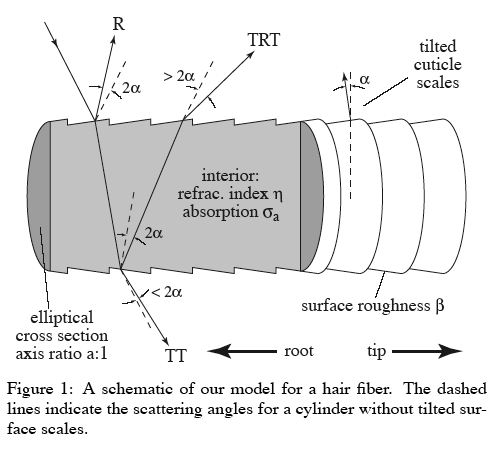
2  Fibers
2.1 Hair fibers and fiber scattering

The fiber is modeled as a dielectric cylinder covered with tilted sacles (the cuticle) and with a pigmented interior (the cortex).

The cones of the R and TRT components shift in opposite directions, causing them to separate into two visually distinguishable highlights. (The R highlight is white and the TRT highlight is colored.)

사용자 삽입 이미지

2.2 Scattering

The bidirectional scattering function S for a fiber (different from the bidirectional reflection distribution function f_r for a surface):
사용자 삽입 이미지

The scattering integral (the curve intensity scattered from an infinitesimal length of fiber):
사용자 삽입 이미지

The presence D in this equation (1) indicates that
a thick fiber intercepts more light, and therefore appears brighter from a distance, than a thin fiber.


3 Scattering measurements
3.1 Incidence plane

As the scattering angle increases, the secondary highlight fades out, while the primary highlight maintains more constant amplitude. Both peaks maintain approximately constant width.

The equal-angle peak


3.2 Normal plane

The hair has a 180 degree rotational symmetry and is bilaterally symmetric in cross section.

The evolution of the peaks as the fiber roatates appears similar to the internal reflection from a transparent elliptical cylinder.


3.3 3D hemispherical measurements
3.3.1 Changes in glints with angle of incidence

The azimuth at which the glints occur changes as a function of incidence angle, with the glints moving toward the incidence plane as the incidence moves from normal to grazing.

3.3.2 Hemispherical scattering


3.4 Summary


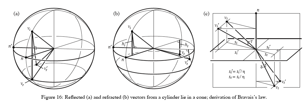
4 Theory of scattering from fibers
4.1 Scattering from cylinders


4.2 Scattering from a circular cross section


사용자 삽입 이미지


posted by maetel
2007. 7. 23. 18:30 Method/VFX
invalid-file

<Programming Graphics Hardware>

Randy Fernando, Mark Harris, Matthias Wloka, Cyril Zeller
NVIDIA Corporation


posted by maetel
2007. 7. 23. 17:46 Method/VFX
invalid-file

<A Simple, Efficient Method for Realistic Animation of Clouds>

Yoshinori Dobashi & Tsuyoshi Okita, Hiroshima City University
Kazufumi Kaneda & Hideo Yamashita, Hiroshima University
Tomoyuki Nishita, University of Tokyo


posted by maetel
2007. 7. 10. 18:44 Cases

http://www.nhk.or.jp/strl/morphovision/

http://www.siggraph.org/s2006/main.php?f=conference&p=etech&s=morpho
The line-shaped images of the digital projector are used as lighting for the high-speed rotating model. The model's high-speed rotation is synchronized with the lighting by a rotating polygon mirror that reflects the line-shaped CG images of the digital projector. The type of lighting is controlled by a touch panel.

Takashi Fukaya
NHK Science and Technical Research Laboratories
fukaya.t-ha (at) nhk.or.jp

Toshio Iwai
Media Artist

Yuko Yamanouchi
NHK Science and Technical Research Laboratories

Ars Electronica Center - Museum der Zukunft
Morphovision, Toshio Iwai (JP)
http://www.aec.at/en/festival2006/program/project.asp?iProjectID=13513

http://360vr.com/Morphovision/

ref.
http://en.wikipedia.org/wiki/DLP
http://en.wikipedia.org/wiki/Cathode_ray_tube

Autostereoscopic light field display
http://gl.ict.usc.edu/Research/3DDisplay/

posted by maetel
2007. 5. 20. 01:20 Method/VFX
http://doi.acm.org/10.1145/357318.357320
invalid-file

Willian T. Reeves <Particle Systems—a Technique for Modeling a Class of Fuzzy Objects>, ACM Transactions on Graphics, Vol.2, no.2, April 1983, Page 91-108


links:
LucanFilm Ltd.
Siggraph: Particle Systems


1
Particle systems model an object as a cloud of primitive particles that define its volume.
Stochastic processes are used to generate and control the many particles within a particle system.

The representation of particel systems :
  1. as clouds of primitive particles that define its volume (not by a set of primitive surface elements)
  2. depending on time (;changing form and moving with the passage of time)
  3. using stochastic processes (to create and change an object's shape and appeareance)

Advantages of the particle system over classical surface-oriented techinique :
  1. A particle is a much simpler primitive than polygon.
    • efficiency of computation time
    • easier removing temporal aliasing  effects (by Motion blurring of fast-moving objects)
  2. The model definition is procedural and is controlled by random numbers.
    • efficiency of human design time (to obtain a highly detailed model)
    • ability to adjust the level of detail (to suit a specific set of viewing parameters)
      • fractal surfaces
  3. It is easier to model "alive" objects changing form over a period of time.

keywords:
image synthesis
stochastic process
    Stochastics
fractal surfaces
procedure
random numbers
stochastic modeling
fractal modeling


2. BASIC MODEL OF PARTICLE SYSTEMS
A particle system is a collection of many minute particles that together represent a fuzzy object. Over a period of time, particles are generated into a system, move and change from within the system, and die from the system.

frame buffer =>
during each interval of time = at a given frame

    2.1 Particle Generation
NParts_f = (MeanParts_sa_f + Rand()*VarParts_sa_f)*ScreenArea
    MeanParts_sa_f = InitialMeanParts_sa + deltaMeanParts_sa*(f-f_0)

    2.2 Particle Attributes
initial position => the origin of a particle system
initial velocity
initial color <= average RGB values and the maximum deviation from them
initial transparency
initial size
shape => a region of newly born random particles about its origin
lifetime
A particle's initial color, transparency and size are determined by
mean values like MeasSpeed, maximum variations like VarSpeed of below:
InitialSpeed = MeanSpeed + Rand()*VarSpeed

사용자 삽입 이미지
More complicated generation shapes based on the law of nature or on chaotic attractors have been envisioned.
    eg. streaked spherical shapes => motion-blur particles

    2.3 Particle Dynamics
    2.4 Particle Extinction
  • when a particle's lifetime reaches zero
  • when the intensity of a particle, calculated from its color and transparency, drops belowa specified threshold
  • when a particle moves more than a given distance in a given direction from the origin of its parent particle system
    2.5 Particle Rendering
        (1) Explosions and fire, the two fuzzy objects we have worekd with the most, are modeled well with the assumption that each particle can be displayed as a point light source. (Other fuzzy objects, such as clouds and water, are not.)
        (2) Since particles do not reflect but emit light, shadows are no longer a problem.
    2.6 Particle Hierarchy


3. USING PARTICLE SYSTEMS TO MODEL A WALL OF FIRE AND EXPLOSIONS
The Genesis Demo sequence from the movie Star Trek II: The Wrath of Khan was generated by the Computer Graphics project of Lucasfilm Ltd.

사용자 삽입 이미지
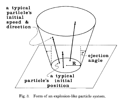
The initial direction of the particles' movement was constrained by the system's ejection angle to fall within the region bounded by the inverted cone. As particles flew upward, the gravity parameter pulled them back down to the planet's surface, giving them a parabolic motion path. The number of particles generated per frame was based on the amount of screen area covered by the particle system.
Varying the mean velocity parameter caused the explosions to be of different heights.
The rate at which a particle's color changed simulated the cooling of a glowing piece of some hypothetical material.

When a motion picture camera is used to film live action at 24 frames per second, the camera shutter typically remains open for 1/50 of a second. The image captured on a frame is actually an integration of approximately half the motion that occurred between successive frames. An object moving quickly appears blurred in the individual still frames.

    ref. Tom Duff

    cf. seed value


4. OTHER PPLICATIONS OF PARTICLE SYSTEMS
    4.1 Fireworks

posted by maetel
2007. 4. 30. 17:52 Computation/Algorithm
The term “particle system” was coined in 1983 by William T. Reeves as he worked to create the “Genesis” effect at the end of the movie, Star Trek II: The Wrath of Khan.

ref.
traer.physics

“A particle system is a collection of many many minute particles that together represent a fuzzy object. Over a period of time, particles are generated into a system, move and change from within the system, and die from the system.”
invalid-file

Willian T. Reeves <Particle Systems—a Technique for Modeling a Class of Fuzzy Objects>

ref.
Siggraph: Particle Systems
Evans & Sutherland @http://www.es.com


invalid-file

Karl Sims <Particle animation and rendering using data parallel computation>

http://doi.acm.org/10.1145/97879.97923
ref.
Karl Sims home page
wikipedia: Karl Sims

invalid-file

Alain Fournier (University of Toronto) & Don Fussell (The University of Texas at Austin) & Loren Carpenter (Lucasfilm) <Computer Rendering of Stochastic Models>

http://doi.acm.org/10.1145/358523.358553


TGLTLSBFSSP: Models
wikipedia: Particle_system
Lucasfilm Ltd. @http://www.lucasfilm.com
GenArts @http://www.genarts.com

'Computation > Algorithm' 카테고리의 다른 글

steering vector  (0) 2007.06.25
Boids  (0) 2007.06.21
Pseudo-random  (0) 2007.04.27
noise  (0) 2007.04.21
Perlin Noise  (0) 2007.04.21
posted by maetel