블로그 이미지
Leeway is... the freedom that someone has to take the action they want to or to change their plans.
maetel

Notice

Recent Post

Recent Comment

Recent Trackback

Archive

calendar

1 2 3 4
5 6 7 8 9 10 11
12 13 14 15 16 17 18
19 20 21 22 23 24 25
26 27 28 29 30 31
  • total
  • today
  • yesterday

Category

'Computer Vision'에 해당되는 글 50건

  1. 2010.02.09 Sola & Monin & Devy & Lemaire, "Undelayed initialization in bearing only SLAM"
  2. 2010.01.25 Kragic & Vincze <Vision for Robotics>
  3. 2010.01.14 RoSEC 2010 winter school
  4. 2009.12.02 Joan Solà - 6DOF SLAM toolbox for Matlab
  5. 2009.11.23 Particle filter for 2D object tracking 연습 5
  6. 2009.11.08 Branislav Kisačanin & Vladimir Pavlović & Thomas S. Huang <Real-Time Vision for Human-Computer Interaction>
  7. 2009.10.29 M. Armstrong & A. Zisserman <Robust object tracking>
  8. 2009.10.27 R. L. Thompson et al. <Providing synthetic views for teleoperation using visual pose tracking in multiple cameras> 1
  9. 2009.10.27 C. Harris & C. Stennett, <Rapid - a video rate object tracker>
  10. 2009.10.26 Somkiat Wangsiripitak & David W Murray <Avoiding moving outliers in visual SLAM by tracking moving objects>
  11. 2009.09.16 Chekhlov et al < Ninja on a Plane: Automatic Discovery of Physical Planes for Augmented Reality Using Visual SLAM>
  12. 2009.08.24 Andrew J. Davison, Ian Reid, Nicholas Molton & Olivier Stasse <MonoSLAM: Real-Time Single Camera SLAM> 1
  13. 2009.08.19 Richard Hartley <In defense of the eight-point algorithm>
  14. 2009.08.18 Five-Point algorithm
  15. 2009.08.05 PTAM test log on Mac OS X 7
  16. 2009.08.04 SLAM related generally
  17. 2009.07.21 임현, 이영삼 <이동로봇의 동시간 위치인식 및 지도작성(SLAM)> 3
  18. 2009.07.14 Trends in Augmented Reality Tracking, Interaction and Display: A Review of Ten Years of ISMAR
  19. 2009.06.08 Photometric stereo 2009-06-07
  20. 2009.03.31 A. J. Davison <Real-time simultaneous localisation and mapping with a single camera>
  21. 2009.03.27 people in SLAM
  22. 2009.02.14 Special Issue on Visual SLAM (IEEE Transactions on Robotics, Vol. 24, No. 5)
  23. 2008.10.16 2.4 Color images & 2.5 Cameras
  24. 2008.09.20 Ch. 6 Segmentation I
  25. 2008.09.10 Ch. 2 The image, its representations and properties
2010. 2. 9. 17:50 Computer Vision

Undelayed initialization in bearing only SLAM


Sola, J.   Monin, A.   Devy, M.   Lemaire, T.  
CNRS, Toulouse, France;

This paper appears in: Intelligent Robots and Systems, 2005. (IROS 2005). 2005 IEEE/RSJ International Conference on
Publication Date: 2-6 Aug. 2005
On page(s): 2499- 2504
ISBN: 0-7803-8912-3
INSPEC Accession Number: 8750433
Digital Object Identifier: 10.1109/IROS.2005.1545392
Current Version Published: 2005-12-05


ref. http://homepages.laas.fr/jsola/JoanSola/eng/bearingonly.html


 기존 SLAM에서 쓰이는 레이저 레인지 스캐너 등 range and bearing 센서 대신 공간에 대한 풍부한 정보를 주는 카메라를 쓰면, 1차원 (인식된 물체까지의 거리 정보, depth)을 잃게 되어 bearing-only SLAM이 된다.

EKF requires Gaussian representations for all the involved random variables that form the map (the robot pose and all landmark's positions). Moreover, their variances need to be small to be able to approximate all the non linear functions with their linearized forms.

두 입력 이미지 프레임 사이에 baseline을 구할 수 있을 만큼 충분한 시점 차가 존재해야 랜드마크의 위치를 결정할 수 있으므로, 이를 확보하기 위한 시간이 필요하게 된다.

http://en.wikipedia.org/wiki/Structure_from_motion
  1. Extract features from images
  2. Find an initial solution for the structure of the scene and the motion of the cameras
  3. Extend the solution and optimise it
  4. Calibrate the cameras
  5. Find a dense representation of the scene
  6. Infer geometric, textural and reflective properties of the scene.

sequential probability ratio test
http://en.wikipedia.org/wiki/Sequential_probability_ratio_test
http://www.agrsci.dk/plb/bembi/africa/sampling/samp_spr.html
http://eom.springer.de/S/s130240.htm

EKF (extended Kalman filter) - inconsistency and divergence
GSF (Gaussian sum filter) - computation load
FIS (Federated Information Sharing)


posted by maetel
2010. 1. 25. 02:50 Computer Vision

Foundations and Trends® in
Robotics

Vol. 1, No. 1 (2010) 1–78
© 2009 D. Kragic and M. Vincze
DOI: 10.1561/2300000001

Vision for Robotics

Danica Kragic1 and Markus Vincze2
1 Centre for Autonomous Systems, Computational Vision and Active Perception Lab, School of Computer Science and Communication, KTH, Stockholm, 10044, Sweden, dani@kth.se
2 Vision for Robotics Lab, Automation and Control Institute, Technische Universitat Wien, Vienna, Austria, vincze@acin.tuwien.ac.at

SUGGESTED CITATION:
Danica Kragic and Markus Vincze (2010) “Vision for Robotics”,
Foundations and Trends® in Robotics: Vol. 1: No. 1, pp 1–78.
http:/dx.doi.org/10.1561/2300000001


Abstract

Robot vision refers to the capability of a robot to visually perceive the environment and use this information for execution of various tasks. Visual feedback has been used extensively for robot navigation and obstacle avoidance. In the recent years, there are also examples that include interaction with people and manipulation of objects. In this paper, we review some of the work that goes beyond of using artificial landmarks and fiducial markers for the purpose of implementing visionbased control in robots. We discuss different application areas, both from the systems perspective and individual problems such as object tracking and recognition.


1 Introduction 2
1.1 Scope and Outline 4

2 Historical Perspective 7
2.1 Early Start and Industrial Applications 7
2.2 Biological Influences and Affordances 9
2.3 Vision Systems 12

3 What Works 17
3.1 Object Tracking and Pose Estimation 18
3.2 Visual Servoing–Arms and Platforms 27
3.3 Reconstruction, Localization, Navigation, and Visual SLAM 32
3.4 Object Recognition 35
3.5 Action Recognition, Detecting, and Tracking Humans 42
3.6 Search and Attention 44

4 Open Challenges 48
4.1 Shape and Structure for Object Detection 49
4.2 Object Categorization 52
4.3 Semantics and Symbol Grounding: From Robot Task to Grasping and HRI 54
4.4 Competitions and Benchmarking 56

5 Discussion and Conclusion 59

Acknowledgments 64
References 65


posted by maetel
2010. 1. 14. 17:27 Footmarks
RoSEC international summer/winter school
Robotics-Specialized Education Consortium for Graduates sponsored by MKE

로봇 특성화 대학원 사업단 주관
2010 RoSEC International Winter School
2010년 1월 11일(월)부터 1월 16일(토)
한양대학교 HIT(한양종합기술연구원) 6층 제1세미나실(606호)


Robot mechanism
Byung-Ju Yi (Hanyang University, Korea)
한양대 휴먼로보틱스 연구실 이병주 교수님  bj@hanyang.ac.kr
- Classification of robotic mechanism and Design consideration of robotic mechanism
- Design Issue and application examples of master slave robotic system
- Trend of robotic mechanism research

Actuator and Practical PID Control
Youngjin Choi (Hanyang University, Korea)
한양대 휴먼로이드 연구실 최영진 교수님 cyj@hanyang.ac.kr
- Operation Principle of DC/RC/Stepping Motors & Its Practice
- PID Control and Tuning
- Stability of PID Control and Application Examples

Coordination of Robots and Humans
Kazuhiro Kosuge (Tohoku University, Japan)
일본 도호쿠 대학 시스템 로보틱스 연구실 고스게 카즈히로 교수님
- Robotics as systems integration
- Multiple Robots Coordination
- Human Robot Coordination and Interaction

Robot Control
Rolf Johansson (Lund University, Sweden)
스웨덴 룬드 대학 로보틱스 연구실 Rolf.Johansson@control.lth.se
- Robot motion and force control
- Stability of motion
- Robot obstacle avoidance

Lecture from Industry or Government
(S. -R. Oh, KIST)

Special Talk from Government
(Y. J. Weon, MKE)

Mobile Robot Navigation
Jae-Bok Song (Korea University, Korea)
고려대 지능로봇 연구실 송재복 교수님 jbsong@korea.ac.kr
- Mapping
- Localization
- SLAM

3D Perception for Robot Vision
In Kyu Park (Inha University, Korea)
인하대 영상미디어 연구실 박인규 교수님 pik@inha.ac.kr
- Camera Model and Calibration
- Shape from Stereo Views
- Shape from Multiple Views

Lecture from Industry or Government
(H. S. Kim, KITECH)

Roboid Studio
Kwang Hyun Park (Kwangwoon University, Korea)
광운대 정보제어공학과 박광현 교수님 akaii@kw.ac.kr
- Robot Contents
- Roboid Framework
- Roboid Component

Software Framework for LEGO NXT
Sanghoon Lee (Hanyang University, Korea)
한양대 로봇 연구실 이상훈 교수님
- Development Environments for LEGO NXT
- Programming Issues for LEGO NXT under RPF of OPRoS
- Programming Issues for LEGO NXT under Roboid Framework

Lecture from Industry or Government
(Robomation/Mobiletalk/Robotis)

Robot Intelligence : From Reactive AI to Semantic AI
Il Hong Suh (Hanyang University, Korea)
한양대 로봇 지능/통신 연구실 서일홍 교수님
- Issues in Robot Intelligence
- Behavior Control: From Reactivity to Proactivity
- Use of Semantics for Robot Intelligence

AI-Robotics
Henrik I. Christensen (Georgia Tech., USA)

-
Semantic Mapping
- Physical Interaction with Robots
- Efficient object recognition for robots

Lecture from Industry or Government
(M. S. Kim, Director of CIR, 21C Frontier Program)

HRI
Dongsoo Kwon (KAIST, Korea)

- Introduction to human-robot interaction
- Perception technologies of HRI
- Cognitive and emotional interaction

Robot Swarm for Environmental Monitoring
Nak Young Chong (JAIST, Japan)

- Self-organizing Mobile Robot Swarms: Models
- Self-organizing Mobile Robot Swarms: Algorithms
- Self-organizing Mobile Robot Swarms: Implementation


posted by maetel
2009. 12. 2. 21:33 Computer Vision
Joan Solà

6DOF SLAM toolbox for Matlab http://homepages.laas.fr/jsola/JoanSola/eng/toolbox.html

References

[1] J. Civera, A.J. Davison, and J.M.M Montiel. Inverse depth parametrization for monocular SLAM. IEEE Trans. on Robotics, 24(5), 2008.

[2] J. Civera, Andrew Davison, and J. Montiel. Inverse Depth to Depth Conversion for Monocular SLAM. In IEEE Int. Conf. on Robotics and Automation, pages 2778 –2783, April 2007.

[3] A. J. Davison. Real-time simultaneous localisation and mapping with a single camera. In Int. Conf. on Computer Vision, volume 2, pages 1403–1410, Nice, October 2003.

[4] Andrew J. Davison. Active search for real-time vision. Int. Conf. on Computer Vision, 1:66–73, 2005.

[5] Andrew J. Davison, Ian D. Reid, Nicholas D. Molton, and Olivier Stasse. MonoSLAM: Real-time single camera SLAM. Trans. on Pattern Analysis and Machine Intelligence, 29(6):1052–1067, June 2007.

[6] Ethan Eade and Tom Drummond. Scalable monocular SLAM. IEEE Int. Conf. on Computer Vision and Pattern Recognition, 1:469–476, 2006.

[7] Thomas Lemaire and Simon Lacroix. Monocular-vision based SLAM using line segments. In IEEE Int. Conf. on Robotics and Automation, pages 2791–2796, Rome, Italy, 2007.

[8] Nicholas Molton, Andrew J. Davison, and Ian Reid. Locally planar patch features for real-time structure from motion. In British Machine Vision Conference, 2004.

[9] J. Montiel, J. Civera, and A. J. Davison. Unified inverse depth parametrization for monocular SLAM. In Robotics: Science and Systems, Philadelphia, USA, August 2006.

[10] L. M. Paz, P. Pini´es, J. Tard´os, and J. Neira. Large scale 6DOF SLAM with stereo-in-hand. IEEE Trans. on Robotics, 24(5), 2008.

[11] J. Sol`a, Andr´e Monin, Michel Devy, and T. Vidal-Calleja. Fusing monocular information in multi-camera SLAM. IEEE Trans. on Robotics, 24(5):958–968, 2008.

[12] Joan Sol`a. Towards Visual Localization, Mapping and Moving Objects Tracking by a Mobile Robot: a Geometric and Probabilistic Approach. PhD thesis, Institut National Polytechnique de Toulouse, 2007.

[13] Joan Sol`a, Andr´e Monin, and Michel Devy. BiCamSLAM: Two times mono is more than stereo. In IEEE Int. Conf. on Robotics and Automation, pages 4795–4800, Rome, Italy, April 2007.

[14] Joan Sol`a, Andr´e Monin, Michel Devy, and Thomas Lemaire. Undelayed initialization in bearing only SLAM. In IEEE/RSJ Int. Conf. on Intelligent Robots and Systems, pages 2499–2504, Edmonton, Canada, 2005.

[15] Joan Sol`a, Teresa Vidal-Calleja, and Michel Devy. Undelayed initialization of line segments in monocular SLAM. In IEEE Int. Conf. on Intelligent Robots and Systems, Saint Louis, USA, 2009. To appear.


slamtb.m


Plucker line (HighLevel/userDataLin.m) http://en.wikipedia.org/wiki/Pl%C3%BCcker_coordinates http://www.cgafaq.info/wiki/Plucker_line_coordinates


direct observation model
http://vismod.media.mit.edu/tech-reports/TR-451/node8.html
inverse observation model
http://vismod.media.mit.edu/tech-reports/TR-451/node9.html
( source: MIT Media Laboratory's Vision and Modeling group )
posted by maetel
2009. 11. 23. 11:48 Computer Vision
to apply Particle filter to object tracking
3차원 파티클 필터를 이용한 물체(공) 추적 (contour tracking) 알고리즘 연습


IplImage* cvRetrieveFrame(CvCapture* capture)

Gets the image grabbed with cvGrabFrame.

Parameter: capture – video capturing structure.

The function cvRetrieveFrame() returns the pointer to the image grabbed with the GrabFrame function. The returned image should not be released or modified by the user. In the event of an error, the return value may be NULL.


Canny edge detection

Canny edge detection in OpenCV image processing functions
void cvCanny(const CvArr* image, CvArr* edges, double threshold1, double threshold2, int aperture_size=3)

Implements the Canny algorithm for edge detection.

Parameters:
  • image – Single-channel input image
  • edges – Single-channel image to store the edges found by the function
  • threshold1 – The first threshold
  • threshold2 – The second threshold
  • aperture_size – Aperture parameter for the Sobel operator (see cvSobel())

The function cvCanny() finds the edges on the input image image and marks them in the output image edges using the Canny algorithm. The smallest value between threshold1 and threshold2 is used for edge linking, the largest value is used to find the initial segments of strong edges.


source cod...ing
// 3-D Particle filter algorithm + Computer Vision exercise
// : object tracking - contour tracking
// lym, VIP Lab, Sogang Univ.
// 2009-11-23
// ref. Probabilistic Robotics: 98p

#include <OpenCV/OpenCV.h> // matrix operations & Canny edge detection
#include <iostream>
#include <cstdlib> // RAND_MAX
#include <ctime> // time as a random seed
#include <cmath>
#include <algorithm>
using namespace std;

#define PI 3.14159265
#define N 100 //number of particles
#define D 3 // dimension of the state

// uniform random number generator
double uniform_random(void) {
   
    return (double) rand() / (double) RAND_MAX;
   
}

// Gaussian random number generator
double gaussian_random(void) {
   
    static int next_gaussian = 0;
    static double saved_gaussian_value;
   
    double fac, rsq, v1, v2;
   
    if(next_gaussian == 0) {
       
        do {
            v1 = 2.0 * uniform_random() - 1.0;
            v2 = 2.0 * uniform_random() - 1.0;
            rsq = v1 * v1 + v2 * v2;
        }
        while(rsq >= 1.0 || rsq == 0.0);
        fac = sqrt(-2.0 * log(rsq) / rsq);
        saved_gaussian_value = v1 * fac;
        next_gaussian = 1;
        return v2 * fac;
    }
    else {
        next_gaussian = 0;
        return saved_gaussian_value;
    }
}

double normal_distribution(double mean, double standardDeviation, double state) {
   
    double variance = standardDeviation * standardDeviation;
   
    return exp(-0.5 * (state - mean) * (state - mean) / variance ) / sqrt(2 * PI * variance);
}
////////////////////////////////////////////////////////////////////////////

// distance between measurement and prediction
double distance(CvMat* measurement, CvMat* prediction)
{
    double distance2 = 0;
    double differance = 0;
    for (int u = 0; u < 3; u++)
    {
        differance = cvmGet(measurement,u,0) - cvmGet(prediction,u,0);
        distance2 += differance * differance;
    }
    return sqrt(distance2);
}

double distanceEuclidean(CvPoint2D64f a, CvPoint2D64f b)
{
    double d2 = (a.x - b.x) * (a.x - b.x) + (a.y - b.y) * (a.y - b.y);
    return sqrt(d2);
}

// likelihood based on multivariative normal distribution (ref. 15p eqn(2.4))
double likelihood(CvMat *mean, CvMat *covariance, CvMat *sample) {
   
    CvMat* diff = cvCreateMat(3, 1, CV_64FC1);
    cvSub(sample, mean, diff); // sample - mean -> diff
    CvMat* diff_t = cvCreateMat(1, 3, CV_64FC1);
    cvTranspose(diff, diff_t); // transpose(diff) -> diff_t
    CvMat* cov_inv = cvCreateMat(3, 3, CV_64FC1);
    cvInvert(covariance, cov_inv); // transpose(covariance) -> cov_inv
    CvMat* tmp = cvCreateMat(3, 1, CV_64FC1);
    CvMat* dist = cvCreateMat(1, 1, CV_64FC1);
    cvMatMul(cov_inv, diff, tmp); // cov_inv * diff -> tmp   
    cvMatMul(diff_t, tmp, dist); // diff_t * tmp -> dist
   
    double likeliness = exp( -0.5 * cvmGet(dist, 0, 0) );
    double bound = 0.0000001;
    if ( likeliness < bound )
    {
        likeliness = bound;
    }
    return likeliness;
//    return exp( -0.5 * cvmGet(dist, 0, 0) );
//    return max(0.0000001, exp(-0.5 * cvmGet(dist, 0, 0)));   
}

// likelihood based on normal distribution (ref. 14p eqn(2.3))
double likelihood(double distance, double standardDeviation) {
   
    double variance = standardDeviation * standardDeviation;
   
    return exp(-0.5 * distance*distance / variance ) / sqrt(2 * PI * variance);
}

int main (int argc, char * const argv[]) {
   
    srand(time(NULL));
   
    IplImage *iplOriginalColor; // image to be captured
    IplImage *iplOriginalGrey; // grey-scale image of "iplOriginalColor"
    IplImage *iplEdge; // image detected by Canny edge algorithm
    IplImage *iplImg; // resulting image to show tracking process   
    IplImage *iplEdgeClone;

    int hours, minutes, seconds;
    double frame_rate, Codec, frame_count, duration;
    char fnVideo[200], titleOriginal[200], titleEdge[200], titleResult[200];
   
    sprintf(titleOriginal, "original");
    sprintf(titleEdge, "Edges by Canny detector");
//    sprintf(fnVideo, "E:/AVCHD/BDMV/STREAM/00092.avi");   
    sprintf(fnVideo, "/Users/lym/Documents/VIP/2009/Nov/volleyBall.mov");
    sprintf(titleResult, "3D Particle filter for contour tracking");
   
    CvCapture *capture = cvCaptureFromAVI(fnVideo);
   
    // stop the process if capture is failed
    if(!capture) { printf("Can NOT read the movie file\n"); return -1; }
   
    frame_rate = cvGetCaptureProperty(capture, CV_CAP_PROP_FPS);
//    Codec = cvGetCaptureProperty( capture, CV_CAP_PROP_FOURCC );
    frame_count = cvGetCaptureProperty( capture, CV_CAP_PROP_FRAME_COUNT);
   
    duration = frame_count/frame_rate;
    hours = duration/3600;
    minutes = (duration-hours*3600)/60;
    seconds = duration-hours*3600-minutes*60;
   
    //  stop the process if grabbing is failed
    //    if(cvGrabFrame(capture) == 0) { printf("Can NOT grab a frame\n"); return -1; }
   
    cvSetCaptureProperty(capture, CV_CAP_PROP_POS_FRAMES, 0); // go to frame #0
    iplOriginalColor = cvRetrieveFrame(capture);
    iplOriginalGrey = cvCreateImage(cvGetSize(iplOriginalColor), 8, 1);
    iplEdge = cvCloneImage(iplOriginalGrey);
    iplEdgeClone = cvCreateImage(cvSize(iplOriginalColor->width, iplOriginalColor->height), 8, 3);
    iplImg = cvCreateImage(cvSize(iplOriginalColor->width, iplOriginalColor->height), 8, 3);   
   
    int width = iplOriginalColor->width;
    int height = iplOriginalColor->height;
   
    cvNamedWindow(titleOriginal);
    cvNamedWindow(titleEdge);
   
    cout << "image width : height = " << width << "  " << height << endl;
    cout << "# of frames = " << frame_count << endl;   
    cout << "capture finished" << endl;   
   
   
    // set the system   
   
    // set the process noise
    // covariance of Gaussian noise to control
    CvMat* transition_noise = cvCreateMat(D, D, CV_64FC1);
    // assume the transition noise
    for (int row = 0; row < D; row++)
    {   
        for (int col = 0; col < D; col++)
        {
            cvmSet(transition_noise, row, col, 0.0);
        }
    }
    cvmSet(transition_noise, 0, 0, 3.0);
    cvmSet(transition_noise, 1, 1, 3.0);
    cvmSet(transition_noise, 2, 2, 0.3);
   
    // set the measurement noise
/*
    // covariance of Gaussian noise to measurement
     CvMat* measurement_noise = cvCreateMat(D, D, CV_64FC1);
     // initialize the measurement noise
     for (int row = 0; row < D; row++)
     {   
        for (int col = 0; col < D; col++)
        {
            cvmSet(measurement_noise, row, col, 0.0);
        }
     }
     cvmSet(measurement_noise, 0, 0, 5.0);
     cvmSet(measurement_noise, 1, 1, 5.0);
     cvmSet(measurement_noise, 2, 2, 5.0); 
 */
    double measurement_noise = 2.0; // standrad deviation of Gaussian noise to measurement
   
    CvMat* state = cvCreateMat(D, 1, CV_64FC1);    // state of the system to be estimated   
//    CvMat* measurement = cvCreateMat(2, 1, CV_64FC1); // measurement of states
   
    // declare particles
    CvMat* pb [N]; // estimated particles
    CvMat* pp [N]; // predicted particles
    CvMat* pu [N]; // temporary variables to update a particle
    CvMat* v[N]; // estimated velocity of each particle
    CvMat* vu[N]; // temporary varialbe to update the velocity   
    double w[N]; // weight of each particle
    for (int n = 0; n < N; n++)
    {
        pb[n] = cvCreateMat(D, 1, CV_64FC1);
        pp[n] = cvCreateMat(D, 1, CV_64FC1);
        pu[n] = cvCreateMat(D, 1, CV_64FC1);   
        v[n] = cvCreateMat(D, 1, CV_64FC1);   
        vu[n] = cvCreateMat(D, 1, CV_64FC1);           
    }   
   
    // initialize the state and particles    
    for (int n = 0; n < N; n++)
    {
        cvmSet(state, 0, 0, 258.0); // center-x
        cvmSet(state, 1, 0, 406.0); // center-y       
        cvmSet(state, 2, 0, 38.0); // radius   
       
//        cvmSet(state, 0, 0, 300.0); // center-x
//        cvmSet(state, 1, 0, 300.0); // center-y       
//        cvmSet(state, 2, 0, 38.0); // radius       
       
        cvmSet(pb[n], 0, 0, cvmGet(state,0,0)); // center-x
        cvmSet(pb[n], 1, 0, cvmGet(state,1,0)); // center-y
        cvmSet(pb[n], 2, 0, cvmGet(state,2,0)); // radius
       
        cvmSet(v[n], 0, 0, 2 * uniform_random()); // center-x
        cvmSet(v[n], 1, 0, 2 * uniform_random()); // center-y
        cvmSet(v[n], 2, 0, 0.1 * uniform_random()); // radius       
       
        w[n] = (double) 1 / (double) N; // equally weighted particle
    }
   
    // initialize the image window
    cvZero(iplImg);   
    cvNamedWindow(titleResult);
   
    cout << "start filtering... " << endl << endl;
   
    float aperture = 3,     thresLow = 50,     thresHigh = 110;   
//    float aperture = 3,     thresLow = 80,     thresHigh = 110;   
    // for each frame
    int frameNo = 0;   
    while(frameNo < frame_count && cvGrabFrame(capture)) {
        // retrieve color frame from the movie "capture"
        iplOriginalColor = cvRetrieveFrame(capture);        
        // convert color pixel values of "iplOriginalColor" to grey scales of "iplOriginalGrey"
        cvCvtColor(iplOriginalColor, iplOriginalGrey, CV_RGB2GRAY);               
        // extract edges with Canny detector from "iplOriginalGrey" to save the results in the image "iplEdge" 
        cvCanny(iplOriginalGrey, iplEdge, thresLow, thresHigh, aperture);

        cvCvtColor(iplEdge, iplEdgeClone, CV_GRAY2BGR);
       
        cvShowImage(titleOriginal, iplOriginalColor);
        cvShowImage(titleEdge, iplEdge);

//        cvZero(iplImg);
       
        cout << "frame # " << frameNo << endl;
       
        double like[N]; // likelihood between measurement and prediction
        double like_sum = 0; // sum of likelihoods
       
        for (int n = 0; n < N; n++) // for "N" particles
        {
            // predict
            double prediction;
            for (int row = 0; row < D; row++)
            {
                prediction = cvmGet(pb[n],row,0) + cvmGet(v[n],row,0)
                            + cvmGet(transition_noise,row,row) * gaussian_random();
                cvmSet(pp[n], row, 0, prediction);
            }
            if ( cvmGet(pp[n],2,0) < 2) { cvmSet(pp[n],2,0,0.0); }
//            cvLine(iplImg, cvPoint(cvRound(cvmGet(pp[n],0,0)), cvRound(cvmGet(pp[n],1,0))),
//             cvPoint(cvRound(cvmGet(pb[n],0,0)), cvRound(cvmGet(pb[n],1,0))), CV_RGB(100,100,0), 1);           
            cvCircle(iplEdgeClone, cvPoint(cvRound(cvmGet(pp[n],0,0)), cvRound(cvmGet(pp[n],1,0))), cvRound(cvmGet(pp[n],2,0)), CV_RGB(255, 255, 0));
//            cvCircle(iplImg, cvPoint(iplImg->width *0.5, iplImg->height * 0.5), 100, CV_RGB(255, 255, 0), -1);
//            cvSaveImage("a.bmp", iplImg);

            double cX = cvmGet(pp[n], 0, 0); // predicted center-y of the object
            double cY = cvmGet(pp[n], 1, 0); // predicted center-x of the object
            double cR = cvmGet(pp[n], 2, 0); // predicted radius of the object           

            if ( cR < 0 ) { cR = 0; }
           
            // measure
            // search measurements
            CvPoint2D64f direction [8]; // 8 searching directions
            // define 8 starting points in each direction
            direction[0].x = cX + cR;    direction[0].y = cY;      // East
            direction[2].x = cX;        direction[2].y = cY - cR; // North
            direction[4].x = cX - cR;    direction[4].y = cY;      // West
            direction[6].x = cX;        direction[6].y = cY + cR; // South
            int cD = cvRound( cR/sqrt(2.0) );
            direction[1].x = cX + cD;    direction[1].y = cY - cD; // NE
            direction[3].x = cX - cD;    direction[3].y = cY - cD; // NW
            direction[5].x = cX - cD;    direction[5].y = cY + cD; // SW
            direction[7].x = cX + cD;    direction[7].y = cY + cD; // SE       
           
            CvPoint2D64f search [8];    // searched point in each direction         
            double scale = 0.4;
            double scope [8]; // scope of searching
   
            for ( int i = 0; i < 8; i++ )
            {
//                scope[2*i] = cR * scale;
//                scope[2*i+1] = cD * scale;
                scope[i] = 6.0;
            }
           
            CvPoint d[8];
            d[0].x = 1;        d[0].y = 0; // E
            d[1].x = 1;        d[1].y = -1; // NE
            d[2].x = 0;        d[2].y = 1; // N
            d[3].x = 1;        d[3].y = 1; // NW
            d[4].x = 1;        d[4].y = 0; // W
            d[5].x = 1;        d[5].y = -1; // SW
            d[6].x = 0;        d[6].y = 1; // S
            d[7].x = 1;        d[7].y = 1; // SE           
           
            int count = 0; // number of measurements
            double dist_sum = 0;
           
            for (int i = 0; i < 8; i++) // for 8 directions
            {
                double dist = scope[i] * 1.5;
                for ( int range = 0; range < scope[i]; range++ )
                {
                    int flag = 0;
                    for (int turn = -1; turn <= 1; turn += 2) // reverse the searching direction
                    {
                        search[i].x = direction[i].x + turn * range * d[i].x;
                        search[i].y = direction[i].y + turn * range * d[i].y;
                       
//                        cvCircle(iplImg, cvPoint(cvRound(search[i].x), cvRound(search[i].y)), 2, CV_RGB(0, 255, 0), -1);
//                        cvShowImage(titleResult, iplImg);
//                        cvWaitKey(100);

                        // detect measurements   
//                        CvScalar s = cvGet2D(iplEdge, cvRound(search[i].y), cvRound(search[i].x));
                        unsigned char s = CV_IMAGE_ELEM(iplEdge, unsigned char, cvRound(search[i].y), cvRound(search[i].x));
//                        if ( s.val[0] > 200 && s.val[1] > 200 && s.val[2] > 200 ) // bgr color               
                        if (s > 250) // bgr color                           
                        { // when the pixel value is white, that means a measurement is detected
                            flag = 1;
                            count++;
//                            cvCircle(iplEdgeClone, cvPoint(cvRound(search[i].x), cvRound(search[i].y)), 3, CV_RGB(200, 0, 255));
//                            cvShowImage("3D Particle filter", iplEdgeClone);
//                            cvWaitKey(1);
/*                            // get measurement
                            cvmSet(measurement, 0, 0, search[i].x);
                            cvmSet(measurement, 1, 0, search[i].y);   
                            double dist = distance(measurement, pp[n]);
*/                            // evaluate the difference between predictions of the particle and measurements
                            dist = distanceEuclidean(search[i], direction[i]);
                            break; // break for "turn"
                        } // end if
                    } // for turn
                    if ( flag == 1 )
                    { break; } // break for "range"
                } // for range
               
                dist_sum += dist; // for all searching directions of one particle 

            } // for i direction
           
            double dist_avg; // average distance of measurements from the one particle "n"
//            cout << "count = " << count << endl;
            dist_avg = dist_sum / 8;
//            cout << "dist_avg = " << dist_avg << endl;
           
//            estimate likelihood with "dist_avg"
            like[n] = likelihood(dist_avg, measurement_noise);
//            cout << "likelihood of particle-#" << n << " = " << like[n] << endl;
            like_sum += like[n];   
        } // for n particle
//        cout << "sum of likelihoods of N particles = " << like_sum << endl;
       
        // estimate states       
        double state_x = 0.0;
        double state_y = 0.0;
        double state_r = 0.0;
        // estimate the state with predicted particles
        for (int n = 0; n < N; n++) // for "N" particles
        {
            w[n] = like[n] / like_sum; // update normalized weights of particles           
//            cout << "w" << n << "= " << w[n] << "  ";               
            state_x += w[n] * cvmGet(pp[n], 0, 0); // center-x of the object
            state_y += w[n] * cvmGet(pp[n], 1, 0); // center-y of the object
            state_r += w[n] * cvmGet(pp[n], 2, 0); // radius of the object           
        }
        if (state_r < 0) { state_r = 0; }
        cvmSet(state, 0, 0, state_x);
        cvmSet(state, 1, 0, state_y);       
        cvmSet(state, 2, 0, state_r);
       
        cout << endl << "* * * * * *" << endl;       
        cout << "estimation: (x,y,r) = " << cvmGet(state,0,0) << ",  " << cvmGet(state,1,0)
        << ",  " << cvmGet(state,2,0) << endl;
        cvCircle(iplEdgeClone, cvPoint(cvRound(cvmGet(state,0,0)), cvRound(cvmGet(state,1,0)) ),
                 cvRound(cvmGet(state,2,0)), CV_RGB(255, 0, 0), 1);

        cvShowImage(titleResult, iplEdgeClone);
        cvWaitKey(1);

   
        // update particles       
        cout << endl << "updating particles" << endl;
        double a[N]; // portion between particles
       
        // define integrated portions of each particles; 0 < a[0] < a[1] < a[2] = 1
        a[0] = w[0];
        for (int n = 1; n < N; n++)
        {
            a[n] = a[n - 1] + w[n];
//            cout << "a" << n << "= " << a[n] << "  ";           
        }
//        cout << "a" << N << "= " << a[N] << "  " << endl;           
       
        for (int n = 0; n < N; n++)
        {   
            // select a particle from the distribution
            int pselected;
            for (int k = 0; k < N; k++)
            {
                if ( uniform_random() < a[k] )               
                {
                    pselected = k;
                    break;
                }
            }
//            cout << "p " << n << " => " << pselected << "  ";       
           
            // retain the selection 
            for (int row = 0; row < D; row++)
            {
                cvmSet(pu[n], row, 0, cvmGet(pp[pselected],row,0));
                cvSub(pp[pselected], pb[pselected], vu[n]); // pp - pb -> vu
            }
        }
       
        // updated each particle and its velocity
        for (int n = 0; n < N; n++)
        {
            for (int row = 0; row < D; row++)
            {
                cvmSet(pb[n], row, 0, cvmGet(pu[n],row,0));
                cvmSet(v[n], row , 0, cvmGet(vu[n],row,0));
            }
        }
        cout << endl << endl ;
       
//      cvShowImage(titleResult, iplImg);  
//        cvWaitKey(1000);       
        cvWaitKey(1);       
        frameNo++;
    }
   
    cvWaitKey();   
   
    return 0;
}


posted by maetel
2009. 11. 8. 16:31 Computer Vision
Branislav Kisačanin & Vladimir Pavlović & Thomas S. Huang
Real-Time Vision for Human-Computer Interaction
(RTV4HCI)
Springer, 2005
(google book's overview)

2004 IEEE CVPR Workshop on RTV4HCI - Papers
http://rtv4hci.rutgers.edu/04/


Computer vision and pattern recognition continue to play a dominant role in the HCI realm. However, computer vision methods often fail to become pervasive in the field due to the lack of real-time, robust algorithms, and novel and convincing applications.

Keywords:
head and face modeling
map building
pervasive computing
real-time detection

Contents:
RTV4HCI: A Historical Overview.
- Real-Time Algorithms: From Signal Processing to Computer Vision.
- Recognition of Isolated Fingerspelling Gestures Using Depth Edges.
- Appearance-Based Real-Time Understanding of Gestures Using Projected Euler Angles.
- Flocks of Features for Tracking Articulated Objects.
- Static Hand Posture Recognition Based on Okapi-Chamfer Matching.
- Visual Modeling of Dynamic Gestures Using 3D Appearance and Motion Features.
- Head and Facial Animation Tracking Using Appearance-Adaptive Models and Particle Filters.
- A Real-Time Vision Interface Based on Gaze Detection -- EyeKeys.
- Map Building from Human-Computer Interactions.
- Real-Time Inference of Complex Mental States from Facial Expressions and Head Gestures.
- Epipolar Constrained User Pushbutton Selection in Projected Interfaces.
- Vision-Based HCI Applications.
- The Office of the Past.
- MPEG-4 Face and Body Animation Coding Applied to HCI.
- Multimodal Human-Computer Interaction.
- Smart Camera Systems Technology Roadmap.
- Index.


RTV4HCI: A Historical Overview
Matthew Turk (mturk@cs.ucsb.edu)
University of California, Santa Barbara
http://www.stanford.edu/~mturk/
http://www.cs.ucsb.edu/~mturk/

The goal of research in real-time vision for human-computer interaction is to develop algorithms and systems that sense and perceive humans and human activity, in order to enable more natural, powerful, and effective computer interfaces.

Computers in the Human Interaction Loop (CHIL)

perceptual interfaces
multimodal interfaces
post-WIMP(windows, icons, menus, pointer) interfaces

implicit user awareness or explicit user control

The user interface
- the software and devices that implement a particular model (or set of models) of HCI

Computer vision technologies must ultimately deliver a better "user experience".

B Shneiderman, Designing the User Interface: Strategies for Effective Human-Computer Interaction, Third Edition, Addison-Wesley, 1998.
: 1) time to learn 2) speed of performance 3) user error rates 4) retention over time 5) subjective satisfaction

- Presence and location (Face and body detection, head and body tracking)
- Identity (Face recognition, gait recognition)
- Expression (Facial feature tracking, expression modeling and analysis)
- Focus of attention (Head/face tracking, eye gaze tracking)
- Body posture and movement (Body modeling and tracking)
- Gesture (Gesture recognition, hand tracking)
- Activity (Analysis of body movement)

eg.
VIDEOPLACE (M W Krueger, Artificial Reality II, Addison-Wesley, 1991)
Magic Morphin Mirror / Mass Hallucinations (T Darrell et al., SIGGRAPH Visual Proc, 1997)

Principal Component Analysis (PCA)
Linear Discriminant Analysis (LDA)
Gabor Wavelet Networks (GWNs)
Active Appearance Models (AAMs)
Hidden Markov Models (HMMs)

Identix Inc.
Viisage Technology Inc.
Cognitec Systems


- MIT Medial Lab
ALIVE system (P Maes et al., The ALIVE system: wireless, full-body interaction with autonomous agents, ACM Multimedia Systems, 1996)
PFinder system (C R Wren et al., Pfinder: Real-time tracking of the human body, IEEE Trans PAMI, pp 780-785, 1997)
KidsRoom project (A Bobick et al., The KidsRoom: A perceptually-based interactive and immersive story environment, PRESENCE: Teleoperators and Virtual Environments, pp 367-391, 1999)


Flocks of Features for Tracking Articulated Objects
Mathias Kolsch (kolsch@nps.edu
Computer Science Department, Naval Postgraduate School, Monterey
Matthew Turk (mturk@cs.ucsb.edu)
Computer Science Department, University of California, Santa Barbara


Visual Modeling of Dynamic Gestures Using 3D Appearance and Motion Features
Guangqi Ye (grant@cs.jhu.edu), Jason J. Corso, Gregory D. Hager
Computational Interaction and Robotics Laboratory
The Johns Hopkins University


Map Building from Human-Computer Interactions
http://groups.csail.mit.edu/lbr/mars/pubs/pubs.html#publications
Artur M. Arsenio (arsenio@csail.mit.edu)
Computer Science and Artificial Intelligence Laboratory
Massachusetts Institute of Technology


Vision-Based HCI Applications
Eric Petajan (eric@f2f-inc.com)
face2face animation, inc.
eric@f2f-inc.com


The Office of the Past
Jiwon Kim (jwkim@cs.washington.edu), Steven M. Seitz (seitz@cs.washington.edu)
University of Washington
Maneesh Agrawala (maneesh@microsoft.com)
Microsoft Research
Proceedings of the 2004 Conference on Computer Vision and Pattern Recognition Workshop (CVPRW'04) Volume 10 - Volume 10  Page: 157   Year of Publication: 2004
http://desktop.google.com
http://grail.cs.washington.edu/projects/office/
http://www.realvnc.com/


Smart Camera Systems Technology Roadmap
Bruce Flinchbaugh (b-flinchbaugh@ti.com)
Texas Instruments

posted by maetel
2009. 10. 29. 19:03 Computer Vision
M. Armstrong and A. Zisserman,
“Robust object tracking,”
in Proc 2nd Asian Conference on Computer Vision, 1995, vol. I.
Springer, 1996, pp. 58–62.


Abstract
We describe an object tracker robust to a number of ambient conditions which often severely degrade performance, for example partial occlusion. The robustness is achieved by describing the object as a set of related geometric primitives (lines, conics, etc.), and using redundant measurements to facilitate the detection of outliers. This improves the overall tracking performance. Results are given for frame rate tracking on image sequences.


posted by maetel
2009. 10. 27. 23:31 Computer Vision
R. L. Thompson, I. D. Reid, L. A. Munoz, and D. W. Murray,
Providing synthetic views for teleoperation using visual pose tracking in multiple cameras,”
IEEE Transactions on Systems, Man and Cybernetics, Part A, vol. 31, no. 1, pp. 43–54, 2001.

Abstract - This paper describes a visual tool for teleoperative experimentation involving remote manipulation and contact tasks. Using modest hardware, it recovers in real-time the pose of moving polyhedral objects, and presents a synthetic view of the scene to the teleoperator using any chosen viewpoint and viewing direction. The method of line tracking introduced by Harris is extended to multiple calibrated cameras, and afforced by robust methods and iterative ltering. Experiments are reported which determine the static and dynamic performance of the vision system, and its use in teleoperation is illustrated in two experiments, a peg in hole manipulation task and an impact control task.


Line tracking 
http://en.wikipedia.org/wiki/Passive_radar#Line_tracking
The line-tracking step refers to the tracking of target returns from individual targets, over time, in the range-Doppler space produced by the cross-correlation processing. A standard Kalman filter is typically used. Most false alarms are rejected during this stage of the processing.


- Three difficulties using the Harris tracker
First it was found to be easily broken by occlusions and changing lighting. Robust methods to mitigate this problem have been investigated monocularly by Armstrong and Zisserman [20], [21]. Although this has a marked effect on tracking performance, the second problem found is that the accuracy of the pose recovered in a single camera was poor, with evident correlation between depth and rotation about axes parallel to the image plane. Maitland and Harris [22] had already noted as much when recovering the pose of a pointing device destined for neurosurgical application [23].
They reported much improved accuracy using two cameras; but the object was stationary, had an elaborate pattern drawn on it and was visible at all times to both cameras. The third difficulty, or rather uncertainty, was that the convergence properties and dynamic performances of the monocular and multicamera methods were largely unreported.


"Harris' RAPiD tracker included a constant velocity Kalman filter."


posted by maetel
2009. 10. 27. 14:40 Computer Vision
Harris' RAPiD
C. Harris and C. Stennett, “Rapid - a video rate object tracker,” in Proc 1st British Machine Vision Conference, Sep 1990, pp. 73–77.


ref.
C. Harris, “Tracking with rigid models,” in Active Vision, A. Blake and A. Yuille, Eds. MIT Press, 1992, pp. 59–73.

RAPID (Real-time Attitude and Position Determination) is a real-time model-based tracking algorithm for a known three dimensional object executing arbitrary motion, and viewed by a single video-camera. The 3D object model consists of selected control points on high contrast edges, which can be surface markings, folds or profile edges.
The use of either an alpha-beta tracker or a Kalman filter permits large object motion to be tracked and produces more stable tracking results. The RAPID tracker runs at video-rate on a standard minicomputer equipped with an image capture board.

alpha-beta tracker
http://en.wikipedia.org/wiki/Alpha_beta_filter

Kalman filter
http://en.wikipedia.org/wiki/Kalman_filter


posted by maetel
2009. 10. 26. 21:35 Computer Vision

Avoiding moving outliers in visual SLAM by tracking moving objects


Wangsiripitak, S.   Murray, D.W.  
Dept. of Eng. Sci., Univ. of Oxford, Oxford, UK;

This paper appears in: Robotics and Automation, 2009. ICRA '09. IEEE International Conference on
Publication Date: 12-17 May 2009
On page(s): 375-380
ISSN: 1050-4729
ISBN: 978-1-4244-2788-8
INSPEC Accession Number: 10748966
Digital Object Identifier: 10.1109/ROBOT.2009.5152290
Current Version Published: 2009-07-06


http://www.robots.ox.ac.uk/~lav//Research/Projects/2009somkiat_slamobj/project.html

Abstract

parallel implementation of monoSLAM with a 3D object tracker
information to register objects to the map's frame
the recovered geometry

I. Introduction

approaches to handling movement in the environment
segmentation between static and moving features
outlying moving points

1) active search -> sparse maps
2) robust methods -> multifocal tensors
3-1) tracking known 3D objects in the scene
  -2) determining whether they are moving
  -3) using their convex hulls to mask out features

"Knowledge that they are occluded rather than unreliable avoids the need to invoke the somewhat cumbersome process of feature deletion, followed later perhaps by unnecessary reinitialization."

[15] H. Zhou and S. Sakane, “Localizing objects during robot SLAM in semi-dynamic environments,” in Proc of the 2008 IEEE/ASME Int Conf on Advanced Intelligent Mechatronics, 2008, pp. 595–601.

"[15] noted that movement is likely to associated with objects in the scene, and classified them according to the likelihood that they would move."

the use of 3D objects for reasoning about motion segmentation and occlusion

occlusion masks

II. Underlying Processes
A. Visual SLAM

Monocular visual SLAM - EKF

idempotent 멱등(冪等)
http://en.wikipedia.org/wiki/Idempotence
Idempotence describes the property of operations in mathematics and computer science that means that multiple applications of the operation do not change the result.

http://en.wikipedia.org/wiki/Quaternions_and_spatial_rotation
http://en.wikipedia.org/wiki/Conversion_between_quaternions_and_Euler_angles
http://en.wikipedia.org/wiki/Quaternion
http://en.wikipedia.org/wiki/Euler_Angles
Berthold K.P. Horn, "Some Notes on Unit Quaternions and Rotation"

"Standard monocular SLAM takes no account of occlusion."

B. Object pose tracking

Harris' RAPiD
[17] C. Harris and C. Stennett, “Rapid - a video rate object tracker,” in Proc 1st British Machine Vision Conference, Sep 1990, pp. 73–77
[20] C. Harris, “Tracking with rigid models,” in Active Vision, A. Blake and A. Yuille, Eds. MIT Press, 1992, pp. 59–73.

"(RAPiD makes the assumption that the pose change required between current and new estimates is sufficiently small, first, to allow a linearization of the solution and, second, to make trivial the problem of inter-image correspondence.) The correspondences used are between predicted point to measured image edge, allowing search in 1D rather than 2D within the image. This makes very sparing use of image data — typically only several hundred pixels per image are addressed."

aperture problem
http://en.wikipedia.org/wiki/Motion_perception
http://focus.hms.harvard.edu/2001/Mar9_2001/research_briefs.html

[21] R. L. Thompson, I. D. Reid, L. A. Munoz, and D. W. Murray, “Providing synthetic views for teleoperation using visual pose tracking in multiple cameras,” IEEE Transactions on Systems, Man and
Cybernetics, Part A, vol. 31, no. 1, pp. 43–54, 2001.
- "Three difficulties using the Harris tracker":
(1)First it was found to be easily broken by occlusions and changing lighting. Robust methods to mitigate this problem have been investigated monocularly by Armstrong and Zisserman. (2)Although this has a marked effect on tracking performance, the second problem found is that the accuracy of the pose recovered in a single camera was poor, with evident correlation between depth and rotation about axes parallel to the image plane. Maitland and Harris had already noted as much when recovering the pose of a pointing device destined for neurosurgical application. They reported much improved accuracy using two cameras; but the object was stationary, had an elaborate pattern drawn on it and was visible at all times to both cameras. (3)The third difficulty, or rather uncertainty, was that the convergence properties and dynamic performances of the monocular and multicamera methods were largely unreported.
(3) : little solution
(2) => [21] "recovered pose using 3 iterations of the pose update cycle per image"
(1) => [21], [22] : search -> matching -> weighting

[22] M. Armstrong and A. Zisserman, “Robust object tracking,” in Proc 2nd Asian Conference on Computer Vision, 1995, vol. I. Springer, 1996, pp. 58–62.

RANSAC
[23] M. Fischler and R. Bolles, “Random sample consensus: a paradigm for model fitting with applications to image analysis and automated cartography,” Communications of the ACM, vol. 24, no. 6, pp. 381–395, June 1981.

Least median of squares as the underlying standard deviation is unknown
[24] P. J. Rousseeuw, “Least median of squares regression,” Journal of the American Statistical Association, vol. 79, no. 388, pp. 871–880, 1984.


III. MonoSLAM with Tracked Objects
A. Information from SLAM to the object tracker


B. Information from the object tracker to SLAM


"The convex hull is uniformly dilated by an amount that corresponds to the projection of the typical change in pose."


posted by maetel
2009. 9. 16. 22:04 Computer Vision
Denis Chekhlov, Andrew Gee, Andrew Calway, Walterio Mayol-Cuevas
Ninja on a Plane: Automatic Discovery of Physical Planes for Augmented Reality Using Visual SLAM
http://dx.doi.org/10.1109/ISMAR.2007.4538840

demo: Ninja on A Plane: Discovering Planes in SLAM for AR

http://www.cs.bris.ac.uk/Publications/pub_master.jsp?id=2000745
posted by maetel
2009. 8. 24. 16:47 Computer Vision
Davison, A. J. and Molton, N. D. 2007.
MonoSLAM: Real-Time Single Camera SLAM.
IEEE Trans. Pattern Anal. Mach. Intell. 29, 6 (Jun. 2007), 1052-1067.
DOI= http://dx.doi.org/10.1109/TPAMI.2007.1049

posted by maetel
2009. 8. 19. 00:35 Computer Vision
In defense of the eight-point algorithm
Hartley, R.I.  
Corp. Res. & Dev., Gen. Electr. Co., Schenectady, NY, USA;
This paper appears in: Pattern Analysis and Machine Intelligence, IEEE Transactions on
Publication Date: June 1997
Volume: 19 , Issue: 6
On page(s): 580 - 593


Zhengyou Zhang

'Computer Vision' 카테고리의 다른 글

Jules Bloomenthal & Jon Rokne "Homogeneous Coordinates"  (0) 2009.08.20
Epipolar geometry - Fundamental matrix  (0) 2009.08.19
Five-Point algorithm  (0) 2009.08.18
UNIX references  (0) 2009.08.17
PTAM to be dissected on OS X  (0) 2009.08.17
posted by maetel
2009. 8. 18. 21:29 Computer Vision
Nistér, D. 2004. An Efficient Solution to the Five-Point Relative Pose Problem. IEEE Trans. Pattern Anal. Mach. Intell. 26, 6 (Jun. 2004), 756-777. DOI= http://dx.doi.org/10.1109/TPAMI.2004.17
An efficient solution to the five-point relative pose problem
Nister, D.  
Sarnoff Corp., Princeton, NJ, USA;

This paper appears in: Pattern Analysis and Machine Intelligence, IEEE Transactions on
Publication Date: June 2004
Volume: 26,  Issue: 6
On page(s): 756-770 An Efficient Solution to the Five-Point Relative Pose Problem

David Nist´er
Sarnoff Corporation
Center for Visualization and Virtual Environments and the Computer Science Department of University of Kentucky


H. Stewenius, C. Engels, and D. Niste. Recent developments on direct relative orientation.
ISPRS Journal of Photogrammetry and Remote Sensing, 60:284-294, June 2006.


Calibrated Fivepoint Solver
http://www.vis.uky.edu/~dnister/Executables/RelativeOrientation/


Dhruv Batra, Bart Nabbe, and Martial Hebert. An Alternative Formulation for the Five Point Relative Pose Problem. IEEE Workshop on Motion and Video Computing 2007 (WMVC '07).
http://www.ece.cmu.edu/~dbatra/research/fivept/fivept.html


Five-Point Motion Estimation Made Easy
Hongdong Li and Richard Hartley (RSISE, The Australian National University. Canberra Research Labs, National ICT Australia.)


preview


SfM = structure from motion
http://en.wikipedia.org/wiki/Structure_from_motion

eight-point algorithm
http://en.wikipedia.org/wiki/Eight-point_algorithm
algorithm used in computer vision to estimate the essential matrix or the fundamental matrix related to a stereo camera pair from a set of corresponding image points

Richard Hartley and Andrew Zisserman (2003). Multiple View Geometry in computer vision. Cambridge University Press.
http://www.robots.ox.ac.uk/~vgg/hzbook/
ch.8 - ch.10

Richard I. Hartley (June 1997). "In Defense of the Eight-Point Algorithm". IEEE Transaction on Pattern Recognition and Machine Intelligence 19 (6): 580–593. doi:10.1109/34.601246.

Richard Szeliski, Microsoft Research
Computer Vision: Algorithms and Applications
ch.7 Structure from Motion

Epipolar geometry - Fundamental matrix


'Computer Vision' 카테고리의 다른 글

Epipolar geometry - Fundamental matrix  (0) 2009.08.19
Richard Hartley <In defense of the eight-point algorithm>  (0) 2009.08.19
UNIX references  (0) 2009.08.17
PTAM to be dissected on OS X  (0) 2009.08.17
PTAM test log on Mac OS X  (7) 2009.08.05
posted by maetel
2009. 8. 5. 14:36 Computer Vision
Oxford 대학  Active Vision Group에서 개발한
PTAM (Parallel Tracking and Mapping for Small AR Workspaces)
http://www.robots.ox.ac.uk/~gk/PTAM/

Questions? E-mail ptam@robots.ox.ac.uk


0. requirements 확인

readme 파일에서 언급하는 대로 프로세서와 그래픽카드를 확인하니

내가 설치할 컴퓨터 사양:
Model Name:    Mac mini
  Model Identifier:    Macmini3,1
  Processor Name:    Intel Core 2 Duo
  Processor Speed:    2 GHz
  Number Of Processors:    1
  Total Number Of Cores:    2
  L2 Cache:    3 MB
  Memory:    1 GB
  Bus Speed:    1.07 GHz
  Boot ROM Version:    MM31.0081.B00

그래픽 카드:
NVIDIA GeForce 9400

"Intel Core 2 Duo processors 2.4GHz+ are fine."이라고 했는데, 2.0이면 되지 않을까? 그래픽 카드는 동일한 것이니 문제 없고.


1. library dependency 확인

1. TooN - a header library for linear algebra
2. libCVD - a library for image handling, video capture and computer vision
3. Gvars3 - a run-time configuration/scripting library, this is a sub-project of libCVD.
셋 다 없으므로,

1-1. TooN 다운로드

TooN (Tom's object oriented Numerics)선형대수 (벡터, 매트릭스 연산)를 위해 Cambridge Machine Intelligence lab에서 개발한 C++ 라이브러리라고 한다.

ref. TooN Documentation (<- 공식 홈보다 정리가 잘 되어 있군.)

다음과 같은 명령으로 다운로드를 받는다.
%% cvs -z3 -d:pserver:anonymous@cvs.savannah.nongnu.org:/sources/toon co TooN

실행 결과:

생성된 TooN 폴더에 들어가서
%%% ./configure

실행 결과:


1-1-1. 더 안정적인(?) 버전을 받으려면

%% cvs -z3 -d:pserver:anonymous@cvs.savannah.nongnu.org:/sources/toon co -D "Mon May 11 16:29:26 BST 2009" TooN

실행 결과:


1-2. libCVD 다운로드

libCVD (Cambridge Video Dynamics)같은 연구실에서 만든 컴퓨터 비전 관련 이미지 처리를 위한 C++ 라이브러리

ref. CVD documentation

%% cvs -z3 -d:pserver:anonymous@cvs.savannah.nongnu.org:/sources/libcvd co -D "Mon May 11 16:29:26 BST 2009" libcvd

실행 결과:


1-3. Gvars3 다운로드

Gvars3 (configuration system library)
 
%% cvs -z3 -d:pserver:anonymous@cvs.savannah.nongnu.org:/sources/libcvd co -D "Mon May 11 16:29:26 BST 2009" gvars3

실행 결과:


2. 다운로드한 기반 라이브러리 설치

2-1. TooN 설치

2-1-1. configure file 실행

configure scripts는 source code를 compile하고 실행시킬 수 있게 만들어 주는 것.

생성된 TooN 폴더에 들어가서
%%% ./configure

실행 결과:

2-1-2. 설치

(TooN은 헤더파일들의 모음이므로 compile이 필요없다.)

%%% sudo make install

실행 결과:
mkdir -p //usr/local/include/TooN
cp *.h //usr/local/include/TooN
cp -r optimization //usr/local/include/TooN/
cp -r internal //usr/local/include/TooN/


2-2. libCVD 설치

2-2-1. configure 파일 실행

생성된 libCVD 폴더에 들어가서
%%% export CXXFLAGS=-D_REENTRANT
%%% ./configure --without-ffmpeg

실행 결과:

2-2-2. documents 생성 (생략해도 되는 듯)

다시 시도했더니
%%% make docs

make: *** No rule to make target `docs'.  Stop.
여전히 안 되는 듯... 아! doxygen을 맥포트로 설치해서 그런가 보다. (데이터베이스가 서로 다르다고 한다.)_M#]


2-2-3. compile 컴파일하기

%%% make

실행 결과:


2-2-4. install 설치하기

%%% sudo make install

실행 결과:


2-3. Gvars3  설치

2-3-1. configure 파일 실행

Gvars3 폴더에 들어가서
%%% ./configure --disable-widgets

실행 결과:


2-3-2. compile 컴파일하기

%%% make

실행 결과:


2-3-3. install 설치하기

%%% sudo make install

mkdir -p //usr/local/lib
cp libGVars3.a libGVars3_headless.a //usr/local/lib
mkdir -p //usr/local/lib
cp libGVars3-0.6.dylib //usr/local/lib
ln -fs  //usr/local/lib/libGVars3-0.6.dylib //usr/local/lib/libGVars3-0.dylib
ln -fs  //usr/local/lib/libGVars3-0.dylib //usr/local/lib/libGVars3.dylib
mkdir -p //usr/local/lib
cp libGVars3_headless-0.6.dylib //usr/local/lib
ln -fs  //usr/local/lib/libGVars3_headless-0.6.dylib //usr/local/lib/libGVars3_headless-0.dylib
ln -fs  //usr/local/lib/libGVars3_headless-0.dylib //usr/local/lib/libGVars3_headless.dylib
mkdir -p //usr/local/include
cp -r gvars3 //usr/local/include


2-4. OS X에서의 컴파일링과 관련하여

ref. UNIX에서 컴파일하기
Porting UNIX/Linux Applications to Mac OS X: Compiling Your Code in Mac OS X


3. PTAM 컴파일

3-1. 해당 플랫폼의 빌드 파일을 PTAM source 디렉토리로 복사

내 (OS X의) 경우, PTAM/Build/OS X에 있는 모든 (두 개의) 파일 Makefile과 VideoSource_OSX.cc를 PTAM 폴더에 옮겼다.

3-2. video source 셋업

카메라에 맞는 video input file을 컴파일하도록 Makefile을 수정해 주어야 한다.
맥의 경우, (아마도 Logitech Quickcam Pro 5000 을 기준으로 하는) 하나의 소스 파일만이 존재하므로 그대로 두면 될 듯.

3-3. video source 추가

다른 비디오 소스들은 libCVD에 클래스로 만들어져 있다고 한다. 여기에 포함되어 있지 않은 경우에는 VideoSource_XYZ.cc 라는 식의 이름을 갖는 파일을 만들어서 넣어 주어야 한다.

3-4. compile

PTAM 폴더에 들어가서
%% make

실행 결과:
g++ -g -O3 main.cc -o main.o -c -I /MY_CUSTOM_INCLUDE_PATH/ -D_OSX -D_REENTRANT
g++ -g -O3 VideoSource_OSX.cc -o VideoSource_OSX.o -c -I /MY_CUSTOM_INCLUDE_PATH/ -D_OSX -D_REENTRANT
g++ -g -O3 GLWindow2.cc -o GLWindow2.o -c -I /MY_CUSTOM_INCLUDE_PATH/ -D_OSX -D_REENTRANT
In file included from OpenGL.h:20,
                 from GLWindow2.cc:1:
/usr/local/include/cvd/gl_helpers.h:38:19: error: GL/gl.h: No such file or directory
/usr/local/include/cvd/gl_helpers.h:39:20: error: GL/glu.h: No such file or directory
/usr/local/include/cvd/gl_helpers.h: In function 'void CVD::glPrintErrors()':
/usr/local/include/cvd/gl_helpers.h:569: error: 'gluGetString' was not declared in this scope
make: *** [GLWindow2.o] Error 1

이 에러 메시지는 다음 링크에서 논의되고 있는 문제와 비슷한 상황인 것 같다.
http://en.allexperts.com/q/Unix-Linux-OS-1064/Compiling-OpenGL-unix-linux.htm


3-4-1. OpenGL on UNIX

PTAM이 OpenGL을 사용하고 있는데, OpenGL이 Mac에 기본으로 설치되어 있으므로 신경쓰지 않았던 부분이다. 물론 system의 public framework으로 들어가 있음을 확인할 수 있다. 그런데 UNIX 프로그램에서 접근할 수는 없는가? (인터넷에서 검색해 보아도 따로 설치할 수 있는 다운로드 링크나 방법을 찾을 수 없다.)

에러 메시지에 대한 정확한 진단 ->
philphys: 일단 OpenGL은 분명히 있을 건데 그 헤더파일과 라이브러리가 있는 곳을 지정해 주지 않아서 에러가 나는 것 같아. 보통 Makefile에 이게 지정되어 있어야 하는데 실행결과를 보니까 전혀 지정되어 있지 않네. 중간에 보면 -I /MY_CUSTOM_INCLUDE_PATH/ 라는 부분이 헤더 파일의 위치를 지정해 주는 부분이고 또 라이브러리는 뒤에 링크할 때 지정해 주게 되어 있는데 거기까지는 가지도 못 했네.
즉, "링커가 문제가 아니라, 컴파일러 옵션에 OpenGL의 헤더파일이 있는 디렉토리를 지정해 주어야 할 것 같다"고 한다.

문제의 Makefile을 들여다보고

Makefile을 다음과 같이 수정하고 (보라색 부분 추가)
COMPILEFLAGS = -I /MY_CUSTOM_INCLUDE_PATH/ -D_OSX -D_REENTRANT -I/usr/X11R6/include/

philphys: /usr/X11R6/include 밑에 GL 폴더가 있고 거기에 필요한 헤더파일들이 모두 들어 있다. 그래서 코드에선 "GL/gl.h" 하는 식으로 explicit하게 GL 폴더를 찾게 된다.

그러고 보면 아래와 같은 설명이 있었던 것이다.
Since the Linux code compiles directly against the nVidia driver's GL headers, use of a different GL driver may require some modifications to the code.

다시 컴파일 하니,
실행 결과:

설치 완료!
두 실행파일 PTAM과 CameraCalibrator이 생성되었다.


3-5. X11R6에 대하여

X11R6 = Xwindow Verion 11 Release 6

Xwindow
X.org


4. camera calibration

CameraCalibrator 파일을 실행시켜 카메라 캘리브레이션을 시도했더니 GUI 창이 뜨는데 연결된 웹캠(Logitech QuickCam Pro 4000)으로부터 입력을 받지 못 한다.

4-0. 증상

CameraCalibrator 실행파일을 열면, 다음과 같은 터미널 창이 새로 열린다.
Last login: Fri Aug  7 01:14:05 on ttys001
%% /Users/lym/PTAM/CameraCalibrator ; exit;
  Welcome to CameraCalibrator
  --------------------------------------
  Parallel tracking and mapping for Small AR workspaces
  Copyright (C) Isis Innovation Limited 2008

  Parsing calibrator_settings.cfg ....
! GUI_impl::Loadfile: Failed to load script file "calibrator_settings.cfg".
  VideoSource_OSX: Creating QTBuffer....
  IMPORTANT
  This will open a quicktime settings planel.
  You should use this settings dialog to turn the camera's
  sharpness to a minimum, or at least so small that no sharpening
  artefacts appear! In-camera sharpening will seriously degrade the
  performance of both the camera calibrator and the tracking system.

그리고 Video란 이름의 GUI 창이 열리는데, 이때 아무런 설정을 바꾸지 않고 그대로 OK를 누르면 위의 터미널 창에 다음과 같은 메시지가 이어지면서 자동 종료된다.
  .. created QTBuffer of size [640 480]
2009-08-07 01:20:57.231 CameraCalibrator[40836:10b] ***_NSAutoreleaseNoPool(): Object 0xf70e2c0 of class NSThread autoreleasedwith no pool in place - just leaking
Stack: (0x96827f0f 0x96734442 0x9673a1b4 0xbc2db7 0xbc7e9a 0xbc69d30xbcacbd 0xbca130 0x964879c9 0x90f8dfb8 0x90e69618 0x90e699840x964879c9 0x90f9037c 0x90e7249c 0x90e69984 0x964879c9 0x90f8ec800x90e55e05 0x90e5acd5 0x90e5530f 0x964879c9 0x94179eb9 0x282b48 0xd9f40xd6a6 0x2f16b 0x2fea4 0x26b6)
! Code for converting from format "Raw RGB data"
  not implemented yet, check VideoSource_OSX.cc.

logout

[Process completed]

그러므로 3-3의 문제 -- set up video source (비디오 소스 셋업) --로 돌아가야 한다.
즉, VideoSource_OSX.cc 파일을 수정해서 다시 컴파일한 후 실행해야 한다.

Other video source classes are available with libCVD. Finally, if a custom video source not supported by libCVD is required, the code for it will have to be put into some VideoSource_XYZ.cc file (the interface for this file is very simple.)

삽질...


4-1. VideoSource_OSX.cc 파일 수정


수정한 VideoSource 파일

터미널 창:
Welcome to CameraCalibrator
  --------------------------------------
  Parallel tracking and mapping for Small AR workspaces
  Copyright (C) Isis Innovation Limited 2008

  Parsing calibrator_settings.cfg ....
  VideoSource_OSX: Creating QTBuffer....
  IMPORTANT
  This will open a quicktime settings planel.
  You should use this settings dialog to turn the camera's
  sharpness to a minimum, or at least so small that no sharpening
  artefacts appear! In-camera sharpening will seriously degrade the
  performance of both the camera calibrator and the tracking system.
>   .. created QTBuffer of size [640 480]
2009-08-13 04:02:50.464 CameraCalibrator[6251:10b] *** _NSAutoreleaseNoPool(): Object 0x9df180 of class NSThread autoreleased with no pool in place - just leaking
Stack: (0x96670f4f 0x9657d432 0x965831a4 0xbc2db7 0xbc7e9a 0xbc69d3 0xbcacbd 0xbca130 0x924b09c9 0x958e8fb8 0x957c4618 0x957c4984 0x924b09c9 0x958eb37c 0x957cd49c 0x957c4984 0x924b09c9 0x958e9c80 0x957b0e05 0x957b5cd5 0x957b030f 0x924b09c9 0x90bd4eb9 0x282b48 0xd414 0xcfd6 0x2f06b 0x2fda4)


4-2. Camera Calibrator 실행


Camera calib is [ 1.51994 2.03006 0.499577 0.536311 -0.0005 ]
  Saving camera calib to camera.cfg...
  .. saved.


5. PTAM 실행


  Welcome to PTAM
  ---------------
  Parallel tracking and mapping for Small AR workspaces
  Copyright (C) Isis Innovation Limited 2008

  Parsing settings.cfg ....
  VideoSource_OSX: Creating QTBuffer....
  IMPORTANT
  This will open a quicktime settings planel.
  You should use this settings dialog to turn the camera's
  sharpness to a minimum, or at least so small that no sharpening
  artefacts appear! In-camera sharpening will seriously degrade the
  performance of both the camera calibrator and the tracking system.
>   .. created QTBuffer of size [640 480]
2009-08-13 20:17:54.162 ptam[1374:10b] *** _NSAutoreleaseNoPool(): Object 0x8f5850 of class NSThread autoreleased with no pool in place - just leaking
Stack: (0x96670f4f 0x9657d432 0x965831a4 0xbb9db7 0xbbee9a 0xbbd9d3 0xbc1cbd 0xbc1130 0x924b09c9 0x958e8fb8 0x957c4618 0x957c4984 0x924b09c9 0x958eb37c 0x957cd49c 0x957c4984 0x924b09c9 0x958e9c80 0x957b0e05 0x957b5cd5 0x957b030f 0x924b09c9 0x90bd4eb9 0x282b48 0x6504 0x60a6 0x11af2 0x28da 0x2766)
  ARDriver: Creating FBO...  .. created FBO.
  MapMaker: made initial map with 135 points.
  MapMaker: made initial map with 227 points.


The software was developed with a Unibrain Fire-i colour camera, using a 2.1mm M12 (board-mount) wide-angle lens. It also runs well with a Logitech Quickcam Pro 5000 camera, modified to use the same 2.1mm M12 lens.

iSight를 Netmate 1394B 9P Bilingual to 6P 케이블로  MacMini에 연결하여 해 보니 더 잘 된다.


'Computer Vision' 카테고리의 다른 글

UNIX references  (0) 2009.08.17
PTAM to be dissected on OS X  (0) 2009.08.17
SLAM related generally  (0) 2009.08.04
Kalman Filter  (0) 2009.07.30
OpenCV 1.0 설치 on Mac OS X  (0) 2009.07.27
posted by maetel
2009. 8. 4. 23:07 Computer Vision
SLAM 전반/기본에 관한 자료

Durrant-Whyte & Bailey "Simultaneous localization and mapping"
http://leeway.tistory.com/667


Søren Riisgaard and Morten Rufus Blas
SLAM for Dummies: A Tutorial Approach to Simultaneous Localization and Mapping
http://leeway.tistory.com/688


Joan Solà Ortega (de l’Institut National Polytechnique de Toulouse, 2007)
Towards visual localization, mapping and moving objects tracking by a mobile robot: A geometric and probabilistic approach
ch3@ http://leeway.tistory.com/628


SLAM summer school
2009 Australian Centre for Field Robotics, University of Sydney
http://www.acfr.usyd.edu.au/education/summerschool.shtml
2006 Department of Engineering Science and Robotics Research Group, Oxford
http://www.robots.ox.ac.uk/~SSS06/Website/index.html
2004 Laboratory for Analysis and Architecture of Systems  (LAAS-CNRS) located in Toulouse
http://www.laas.fr/SLAM/
2002 Centre for Autonomous Systems
Numerical Analysis and Computer Science
Royal Institute of Technology
, Stockholm
http://www.cas.kth.se/SLAM/


http://www.doc.ic.ac.uk/%7Eajd/Scene/Release/monoslamtutorial.pdf
Oxford 대학 Active Vision LabVisual Information Processing (VIP) Research Group에서 개발한 SceneLib tutorial인데, Monocular Single Camera를 사용한 SLAM의 기본 개념을 정리해 놓았다.

'Computer Vision' 카테고리의 다른 글

PTAM to be dissected on OS X  (0) 2009.08.17
PTAM test log on Mac OS X  (7) 2009.08.05
Kalman Filter  (0) 2009.07.30
OpenCV 1.0 설치 on Mac OS X  (0) 2009.07.27
cameras on mac os x  (0) 2009.07.27
posted by maetel
2009. 7. 21. 16:16 Computer Vision
임현, 이영삼 (인하대 전기공학부)
이동로봇의 동시간 위치인식 및 지도작성(SLAM)
제어 로봇 시스템 학회지 제15권 제2호 (2009년 6월)
from kyu


> definition
mapping: 환경을 인식가능한 정보로 변환하고
localization: 이로부터 자기 위치를 추정하는 것

> issues
- uncertainty <= sensor
- data association (데이터 조합): 차원이 높은 센서 정보로부터 2-3차원 정도의 정보를 추려내어 이를 지속적으로 - 대응시키는 것
- 관찰된 특징점 자료들을 효율적으로 관리하는 방법


> localization (위치인식)
: 그 위치가 미리 알려진 랜드마크를 관찰한 정보를 토대로 자신의 위치를 추정하는 것
: 초기치 x0와 k-1시점까지의 제어 입력, 관측벡터와 사전에 위치가 알려진 랜드마크를 통하여 매 k시점마다 로봇의 위치를 추정하는 것
- 로봇의 위치추정의 불확실성은 센서의 오차로부터 기인함.

> mapping (지도작성)
: 기준점과 상대좌표로 관찰된 결과를 누적하여 로봇이 위치한 환경을 모델링하는 것
: 위치와 관측정보 그리고 제어입력으로부터 랜드마크 집합을 추정하는 것
- 지도의 부정확성은 센서의 오차로부터 기인함.

> Simultaneous Localization and Mapping (SLAM, 동시간 위치인식 및 지도작성)
: 위치한 환경 내에서 로봇의 위치를 추정하는 것
: 랜드마크 관측벡터와 초기값 그리고 적용된 모든 제어입력이 주어진 상태에서 랜드마크의 위치와 k시점에서의 로봇 상태벡터 xk의 결합확률
- 재귀적 방법 + Bayes 정리
- observation model (관측 모델) + motion model (상태 공간 모델, 로봇의 움직임 모델)
- motion model은 상태 천이가 Markov 과정임을 의미함. (현재 상태는 오직 이전 상태와 입력 벡터로서 기술되고, 랜드마크 집합과 관측에 독립임.)
- prediction (time-update) + correction (measurement-update)
- 불확실성은 로봇 주행거리계와 센서 오차로부터 유발됨.


conditional Bayes rule
http://en.wikipedia.org/wiki/Bayes%27_theorem
 P(A|B \cap C) = \frac{P(A \cap B \cap C)}{P(B \cap C)} = \frac{P(B|A \cap C) \, P(A|C) \, P(C)}{P(C) \, P(B|C)} = \frac{P(B|A \cap C) \, P(A|C)}{P(B|C)}\,.

Markov process

total probability theorem: "law of alternatives"
http://en.wikipedia.org/wiki/Total_probability_theorem
\Pr(A)=\sum_{n} \Pr(A\cap B_n)\,
\Pr(A)=\sum_{n} \Pr(A\mid B_n)\Pr(B_n).\,

> Extended Kalman filter (EKF, 확장 칼만 필터)


http://en.wikipedia.org/wiki/Ground_truth

posted by maetel
2009. 7. 14. 21:23 Computer Vision
ISMAR 2008
7th IEEE/ACM International Symposium on Mixed and Augmented Reality, 2008


Proceedings
State of the Art Report

Trends in Augmented Reality Tracking, Interaction and Display
: A Review of Ten Years of ISMAR
Feng Zhou (Center for Human Factors and Ergonomics, Nanyang Technological University, Singapore)
Henry Been-Lirn Duh (Department of Electrical and Computer Engineering/Interactive and Digital Media Institute, National University of Singapore)
Mark Billinghurst (The HIT Lab NZ, University of Canterbury, New Zealand)


Tracking

1. Sensor-based tracking -> ubiquitous tracking and dynamic data fusion

2. Vision-based tracking: feature-based and model-based
1) feature-based tracking techniques:
- To find a correspondence between 2D image features and their 3D world frame coordinates.
- Then to find the camera pose from projecting the 3D coordinates of the feature into the observed 3D image coordinates and minimizing the distance to their corresponding 3D features.

2) model-based tracking techniques:
- To explicitly use a model of the features of tracked objects such as a CAD model or 2D template of the object based on the distinguishable features.
- A visual serving approach adapted from robotics to calculate camera pose from a range of model features (line, circles, cylinders and spheres)
- knowledge about the scene by predicting hidden movement of the object and reducing the effects of outlier data

3. Hybrid tracking
- closed-loop-type tracking based on computer vision techonologies
- motion prediction
- SFM (structure from motion)
- SLAM (simultaneous localization and mapping)


Interaction and User Interfaces

1. Tangible
2. Collaborative
3. Hybrid


Display

1. See-through HMDs
1) OST = optical see-through
: the user to see the real world with virtual objects superimposed on it by optical or video technologies
2) VST = video see-through
: to display graphical infromation directly on real objects or even daily surfaces in everyday life
2. Projection-based Displays
3. Handheld Displays


Limitations of AR

> tracking
1) complexity of the scene and the motion of target objects, including the degrees of freedom of individual objects and their represenation
=> correspondence analysis: Kalman filters, particle filters.
2) how to find distinguishable objects for "markers" outdoors

> interaction
ergonomics, human factors, usability, cognition, HCI (human-computer interaction)

> AR displays
- HMDs - limited FOV, image distortions,
- projector-based displays - lack mobility, self-occlusion
- handheld displays - tracking with markers to limit the work range

Trends and Future Directions

1. Tracking
1) RBPF (Rao-Blackwellized particle filters) -> automatic recognition systems
2) SLAM, ubiquitous tracking, sensor network -> free from prior knowledge
3) pervasive middleware <- information fusion algorithms

2. Interaction and User Interfaces
"Historically, human knowledge, experience and emotion are expressed and communicated in words and pictures. Given the advances in interface and data capturing technology, knowledge, experience and emotion might now be presented in the form of AR content."

3. AR Displays


Studierstube Augmented Reality Project
: software framework for the development of Augmented Reality (AR) and Virtual Reality applications
Graz University of Technology (TU Graz)

Sharedspace project
The Human Interface Technology Laboratory (HITLab) at the University ofWashington and ATR Media Integration & Communication in Kyoto,Japan join forces at SIGGRAPH 99

The Invisible Train - A Handheld Augmented Reality Game

AR Tennis
camera based tracking on mobile phones in face-to-face collaborative Augmented Reality

Emmie - Environment Management for Multi-User Information Environments

VITA: visual interaction tool for archaeology

HMD = head-mounted displays

OST = optical see-through

VST = video see-through

ELMO: an Enhanced optical see-through display using an LCD panel for Mutual Occlusion

FOV
http://en.wikipedia.org/wiki/Field_of_view_(image_processing)

HMPD = head-mounted projective displays

The Touring Machine

MARS - Mobile Augmented Reality Systems
    
Klimt - the Open Source 3D Graphics Library for Mobile Devices

AR Kanji - The Kanji Teaching application


references  
Ronald T. Azuma  http://www.cs.unc.edu/~azuma/
A Survey of Augmented Reality. Presence: Teleoperators and Virtual Environments 6, 4 (August 1997), 355 - 385. Earlier version appeared in Course Notes #9: Developing Advanced Virtual Reality Applications, ACM SIGGRAPH '95 (Los Angeles, CA, 6-11 August 1995), 20-1 to 20-38.

Ronald Azuma, Yohan Baillot, Reinhold Behringer, Steven Feiner,Simon Julier, Blair MacIntyre
Recent Advances in Augmented Reality.IEEE Computer Graphics and Applications 21, 6 (Nov/Dec 2001),34-47.

Ivan E. Sutherland
The Ultimate Display, IFIP `65, pp. 506-508, 1965

Kato, H.   Billinghurst, M.   Poupyrev, I.   Imamoto, K.   Tachibana, K.   Hiroshima City Univ.
Virtual object manipulation on a table-top AR environment

Sandor, C., Olwal, A., Bell, B., and Feiner, S. 2005.
Immersive Mixed-Reality Configuration of Hybrid User Interfaces.
In Proceedings of the 4th IEEE/ACM international Symposium on Mixed and Augmented Reality(October 05 - 08, 2005). Symposium on Mixed and Augmented Reality. IEEEComputer Society, Washington, DC, 110-113. DOI=http://dx.doi.org/10.1109/ISMAR.2005.37

An optical see-through display for mutual occlusion with a real-time stereovision system
Kiyoshi Kiyokawa, Yoshinori Kurata and Hiroyuki Ohno
Computers & Graphics Volume 25, Issue 5, October 2001, Pages 765-779

Bimber, O., Fröhlich, B., Schmalstieg, D., and Encarnação, L. M. 2005.
The virtual showcase. In ACM SIGGRAPH 2005 Courses (Los Angeles, California, July 31 - August 04, 2005). J. Fujii, Ed. SIGGRAPH '05. ACM, New York, NY, 3. DOI= http://doi.acm.org/10.1145/1198555.1198713

Bimber, O., Wetzstein, G., Emmerling, A., and Nitschke, C. 2005.
Enabling View-Dependent Stereoscopic Projection in Real Environments. In Proceedings of the 4th IEEE/ACM international Symposium on Mixed and Augmented Reality (October 05 - 08, 2005). Symposium on Mixed and Augmented Reality. IEEE Computer Society, Washington, DC, 14-23. DOI= http://dx.doi.org/10.1109/ISMAR.2005.27

Cotting, D., Naef, M., Gross, M., and Fuchs, H. 2004.
Embedding Imperceptible Patterns into Projected Images for Simultaneous Acquisition and Display. In Proceedings of the 3rd IEEE/ACM international Symposium on Mixed and Augmented Reality (November 02 - 05, 2004). Symposium on Mixed and Augmented Reality. IEEE Computer Society, Washington, DC, 100-109. DOI= http://dx.doi.org/10.1109/ISMAR.2004.30

Ehnes, J., Hirota, K., and Hirose, M. 2004.
Projected Augmentation - Augmented Reality using Rotatable Video Projectors. In Proceedings of the 3rd IEEE/ACM international Symposium on Mixed and Augmented Reality (November 02 - 05, 2004). Symposium on Mixed and Augmented Reality. IEEE Computer Society, Washington, DC, 26-35. DOI= http://dx.doi.org/10.1109/ISMAR.2004.47

Arango, M., Bahler, L., Bates, P., Cochinwala, M., Cohrs, D., Fish, R., Gopal, G., Griffeth, N., Herman, G. E., Hickey, T., Lee, K. C., Leland, W. E., Lowery, C., Mak, V., Patterson, J., Ruston, L., Segal, M., Sekar, R. C., Vecchi, M. P., Weinrib, A., and Wuu, S. 1993.
The Touring Machine system. Commun. ACM 36, 1 (Jan. 1993), 69-77. DOI= http://doi.acm.org/10.1145/151233.151239

Gupta, S. and Jaynes, C. 2006.
The universal media book: tracking and augmenting moving surfaces with projected information. In Proceedings of the 2006 Fifth IEEE and ACM international Symposium on Mixed and Augmented Reality (Ismar'06) - Volume 00 (October 22 - 25, 2006). Symposium on Mixed and Augmented Reality. IEEE Computer Society, Washington, DC, 177-180. DOI= http://dx.doi.org/10.1109/ISMAR.2006.297811


Klein, G. and Murray, D. 2007.
Parallel Tracking and Mapping for Small AR Workspaces. In Proceedings of the 2007 6th IEEE and ACM international Symposium on Mixed and Augmented Reality - Volume 00 (November 13 - 16, 2007). Symposium on Mixed and Augmented Reality. IEEE Computer Society, Washington, DC, 1-10. DOI= http://dx.doi.org/10.1109/ISMAR.2007.4538852

Neubert, J., Pretlove, J., and Drummond, T. 2007.
Semi-Autonomous Generation of Appearance-based Edge Models from Image Sequences. In Proceedings of the 2007 6th IEEE and ACM international Symposium on Mixed and Augmented Reality - Volume 00 (November 13 - 16, 2007). Symposium on Mixed and Augmented Reality. IEEE Computer Society, Washington, DC, 1-9. DOI= http://dx.doi.org/10.1109/ISMAR.2007.4538830

posted by maetel
2009. 6. 8. 15:17 Computer Vision
To do: Surface shape reconstruction
: Least squares surface fitting


- path integration
- least squares optimization
- Lucas-Kanade algorithm

http://mathworld.wolfram.com/LeastSquaresFitting.html


 /* We want to solve Mz = v in a least squares sense.  The
    solution is M^T M z = M^T v.  We denote M^T M as A and
    M^T v as b, so A z = b. */

 CMatrixSparse<double> A(M.mTm());
    assert(A.isSymmetric());
    CVector<double> r = A*z;  /* r is the "residual error" */
    CVector<double> b(v*M);

 // solve the equation A z = b
    solveQuadratic<double>(A,b,z,300,CGEPSILON);

 // copy the depths back from the vector z into the image depths
    copyDepths(z,zind,depths);


template <class T>
double solveQuadratic(const CMatrixSparse<T> & A, const CVector<T> & b,
       CVector<T> & x,int i_max, double epsilon)
{
  //my conjugate gradient solver for .5*x'*A*x -b'*x, based on the
  // tutorial by Jonathan Shewchuk  (or is it +b'*x?)
 
  printf("Performing conjugate gradient optimization\n");

  int numvars = x.Length();
  assert(b.Length() == numvars && A.rows() == numvars &&
  A.columns() == numvars);

  int i =0;

  CVector<T> r = b-A*x;
  CVector<T> d= r;
  double delta_new = r.dot(r);
  double delta_0 = delta_new;

  int numrecompute = (int)floor(sqrt(float(numvars)));
  //int numrecompute = 1;
  printf("numrecompute = %d\n",numrecompute);

  printf("delta_new = %f\n", delta_new);
  while (i < i_max && delta_new > epsilon)//epsilon*epsilon*delta_0)
    {
      printf("Step %d, delta_new = %f      \r",i,delta_new);
     
      CVector<T> q = A*d;
      double alpha = delta_new/d.dot(q);
      x.daxpy(d,alpha); //      x += d*alpha;
      if (i % numrecompute == 0)
 {
   //   printf(" ** recompute\n");
   r = b-A*x;
 }
      else
 r.daxpy(q,-alpha); //  r = r-q*alpha;
      double delta_old = delta_new;
      delta_new = r.dot(r);
      double beta = delta_new/delta_old;
      d = r+d*beta;
      i++;
    }

  return delta_new;
  //  return delta_new <= epsilon;
  //  return !(delta_new > epsilon*epsilon*delta_0);
}


'Computer Vision' 카테고리의 다른 글

Reinhard Diestel <Graph Theory>  (0) 2009.06.16
photometric stereo 2009-06-10  (0) 2009.06.10
Photometric stereo 2009-06-05  (0) 2009.06.05
photometric stereo 2009-05-15  (0) 2009.05.15
Criminisi, Reid, Zisserman <Single View Metrology>  (0) 2009.05.06
posted by maetel
2009. 3. 31. 21:10 Computer Vision

Real-time simultaneous localisation and mapping with a single camera

Davison, A.J.  
Dept. of Eng. Sci., Oxford Univ., UK;

This paper appears in: Computer Vision, 2003. Proceedings. Ninth IEEE International Conference on
Publication Date: 13-16 Oct. 2003
On page(s): 1403-1410 vol.2
ISBN: 0-7695-1950-4
INSPEC Accession Number: 7971070
Digital Object Identifier: 10.1109/ICCV.2003.1238654
Current Version Published: 2008-04-03


posted by maetel
2009. 3. 27. 21:05 Computer Vision

Hugh F. Durrant-Whyte, Australian Centre for Field Robotics
http://en.wikipedia.org/wiki/Hugh_F._Durrant-Whyte

John J. Leonard, Center for Ocean Engineering, MIT

Sebastian Thrun, Stanford Artificial Intelligence Laboratory, Stanford University
http://en.wikipedia.org/wiki/Sebastian_Thrun

David Nistér, Center for Visualization and Virtual Environments, University of Kentucky

Ethan Eade, Machine Intelligence lab, Engineering Department, Cambridge University

Tom Drummond, Machine Intelligence Laboratory, Engineering Department, Cambridge University

Javier Civera, Departamento de Informática e Ingeniería de Sistemas, Universidad de Zaragoza

Andrew J. Davison, Reader in Robot Vision at the Department of Computing, Imperial College London

Jose Maria Martinez Montiel, Robotics and Real Time Group, Universidad de Zaragoza

Robert Castle, Active Vision Laboratory, Robotics Research Group, Oxford University

임현Embedded control system 연구실, 전기공학부, 인하대학교

김정호, Robotics and Computer Vision 연구실 (권인소), 한국과학기술원

labs
 
Active Vision Goup, Robotics Research Group, Engineering Department, Oxford University

Computer Vision & Robotics Group, Machine Intelligence Laboratory, Department of Engineering, University of Cambridge

Image Information Processing Lab 영상정보처리연구실 (홍기상), 포항공대

Intelligent Control and Systems Lab 지능제어 및 시스템 연구실 (김상우), 포항공대


posted by maetel
2009. 2. 14. 17:27 Computer Vision
IEEE Transactions on Robotics, Volume 24, Number 5, October 2008
: Visual SLAM Special Issue

Guest Editorial: Special Issue on Visual SLAM


simultaneous localization mapping (SLAM)
in autonomous mobile robotics
using laser range-finder sensors
to build 2-D maps of planar environments

SLAM with standard cameras:
feature detection
data association
large-scale state estimation

SICK laser scanner


Kalman filter
Particle filter
submapping

http://en.wikipedia.org/wiki/Particle_filter
particle filter = sequential Monte Carlo methods (SMC)


http://en.wikipedia.org/wiki/Image_registration
the process of transforming the different sets of data into one coordinate system


http://en.wikipedia.org/wiki/Simultaneous_localization_and_mapping
the process of creating geometrically accurate maps of the environment
to build up a map within an unknown environment while at the same time keeping track of their current position

R.C. Smith and P. Cheeseman (1986)

Hugh F. Durrant-Whyte (early 1990s)

Sebastian Thrun

mobile robotics
autonomous vehicle

한국로봇산업협  http://www.korearobot.or.kr/


posted by maetel
2008. 10. 16. 20:42 @GSMC/박래홍: Computer Vision

2.4 Color images

2.4.1 Physics of color


2.4.2 Color perceived by humans


XYZ color space
http://en.wikipedia.org/wiki/Xyz_color_space


color matching functions
: numerical description of the chromatic response of the observer


color gamut:
subsapce of colors perceived by humans

http://en.wikipedia.org/wiki/Gamut
Digitizing a photograph, converting a digitized image to a different color space, or outputting it to a given medium using a certain output device generally alters its gamut, in the sense that some of the colors in the original are lost in the process.


37p

2.4.3 Color spaces

http://en.wikipedia.org/wiki/Color_space

http://en.wikipedia.org/wiki/Rounding_error

(1) RGB color space
- CRT
- relative color standard
- additive color mixing
- sRGB, Adobe RGB, Adobe Wide Gamut RGB

http://en.wikipedia.org/wiki/RGB_color_space
The complete specification of an RGB color space also requires a white point chromaticity and a gamma correction curve.


(2) YIQ color space
- additive color mixing
- luminance (the perceived energy ot a light source)

http://en.wikipedia.org/wiki/YIQ
The Y component represents the luma information, and is the only component used by black-and-white television receivers. I and Q represent the chrominance information.

(3) YUV color space

http://en.wikipedia.org/wiki/YUV
Y' stands for the luma component (the brightness) and U and V are the chrominance (color) components.


(4) CMY color space
- subtractive color mixing (in printing process)
- sets of inks, substrates, and press characteristics

http://en.wikipedia.org/wiki/CMYK_color_model
masking certain colors on the typically white background (that is, absorbing particular wavelengths of light)


(5) HSV color space
- Hue, Saturation, Value (; HSB, Hue, Saturation, Brightness ; HSI; Hue, Saturation, Intensity)
- => image enhancement algorithms

http://en.wikipedia.org/wiki/HSL_and_HSV
Because HSL and HSV are simple transformations of device-dependent RGB, the color defined by a (h, s, l) or (h, s, v) triplet depends on the particular color of red, green, and blue “primaries” used. Each unique RGB device therefore has unique HSL and HSV spaces to accompany it. An (h, s, l) or (h, s, v) triplet can however become definite when it is tied to a particular RGB color space, such as sRGB.


39p

2.4.4 Palette images


palette images; indexed images

lookup table; color table; color map; index register; palette

The number of colors in the image exceeds the number of entries in the lookup table and a subset of colors has to be chosen, and a loss of information occurs.

vector quantization (-> 14.4)
1) to check which colors appear in the image by creating histograms for all three color components
2) to quantize them to provide more shades for colors which occur in the image frequently
3) to find the nearest color in the lookup table to represent the color 

=> to analyze large multi-dimensional datasets

http://en.wikipedia.org/wiki/Vector_quantization

http://en.wikipedia.org/wiki/Cluster_analysis
Clustering is the classification of objects into different groups, or more precisely, the partitioning of a data set into subsets (clusters), so that the data in each subset (ideally) share some common trait - often proximity according to some defined distance measure.

http://en.wikipedia.org/wiki/K_means
The k-means algorithm is an algorithm to cluster n objects based on attributes into k partitions, k < n. It is similar to the expectation-maximization algorithm for mixtures of Gaussians in that they both attempt to find the centers of natural clusters in the data.


pseudocolor


Palette selection depends on the semantics of the image and is an interactive process.


2.4.5 Color constancy

The same surface color under diffrent illumination
 
> color compensations
- to scale the sensitivity of each sensor type
=> automatic white balancing
- to assume that the brightest point in the image has the color of the illumination


2.5 Cameras: an overview


2.5.1 Photosensitive sensors

> photosensitive sensors in cameras
(1) photo-emission

photoelectric effect (; Hertz Effect)
http://en.wikipedia.org/wiki/Photoelectric_effect

photomultipliers
vacuum tube TV cameras

(2) photovoltanic

http://en.wikipedia.org/wiki/Solar_cell

photodiode
night vision camera
photoresistor
Schottky photodiode


> semiconductor photoresistive sensors
(1) CCDs (charge-coupled devices)
- arranged into a matrix-like grid of pixels (CCD chip)
- blooming effect
- shift registers
- SNR fropped

(2) CMOS (complementary metal oxide semiconductor)
- all of the pixel area devoted to light capture
- matrix-like sensors


2.5.2 A monochromatic camera

2.5.3 A color camera


2.6 Summary

'@GSMC > 박래홍: Computer Vision' 카테고리의 다른 글

Ch.10 Image Understanding  (0) 2008.12.15
Ch.9 Object Recognition  (0) 2008.11.25
Ch. 6 Segmentation I  (0) 2008.09.20
Ch. 2 The image, its representations and properties  (0) 2008.09.10
Ch.1 Introduction  (0) 2008.09.04
posted by maetel
175p

> to divide an image into parts with a strong correlation with objects or areas of the real world contained in the image
- complete segmentation
: lower-level (context independent processing using no object-related model)
- partial segmentation
: dividing an image into separate regions that are homogeneous with respect to a chosen property (such as brightness, color, reflectivity, texture, etc)

http://en.wikipedia.org/wiki/Segmentation_(image_processing)

> segmentation methods
(1) global knowledge - a histogram of image features
(2) edge-based segmentations <- edge detection
(3) region-based segmentations <- region growing

eg. (2) + (3) => a region adjacency graph
http://www.mathworks.com/matlabcentral/fileexchange/loadFile.do?objectId=16938&objectType=FILE

cf. topological data structure


176p
6.1 Thresholding

Thresholding
: the transformation of an input image to an output (segmented) binary image

interactive threshold selection / threshold detection method

> gray-level
global thresholding
using a single threshold for the whole image
adaptive thresholding
using variable thresholds, dep. on local image characteristics
(<- non-uniform lighting, non-uniform input device parameters)
band thresholding
using limited gray-level subsets
(-> blood cell segmentations, border detector)
+ multiple thresholds
semi-thresholding
human-assisted analysis

> gradient, a local texture property, an image decomposition criterion

http://en.wikipedia.org/wiki/Thresholding_(image_processing)

179p

6.1.1 Threshold detection methods

p-tile thresholding
<- prior information about area ratios

histogram shape analysis
: gray values between the two peaks probably result from border pixels between objects and background 

multi-thresholding

mode method
: to find the highest local maxima first and detect the threshold as a minimum between them

to build a histogram with a better peak-to-valley ratio
(1) to weight histogram contributions to suppress the influence of pixels with a high image gradient
(2) to use only high-gradient pixels to form the gray-level histogram which should be unimodal corresponding to the gray-level of borders

histogram transformation

hitogram concavity analysis

entropic methods

relaxation methods

multi-thresholding methods

ref. A survey of thresholding techniques
Computer Vision, Graphics, and Image Processing, 1988
PK Sahoo, S Soltani, AKC Wong, YC Chen


180p

6.1.2 Optimal thresholding

optimal thresholding
: using a weighted sum of two or more probability densities with normal distribution

"estimating normal distribution parameters together with the uncertainty that the distribution may be considered normal"

ref.
Rosenfeld and Kak, 1982
Gonzalez and Wintz, 1987

minimization of variance of the histogram
sum of square errors
spatial entropy
average clustering

ref. An analysis of histogram-based thresholding algorithms
CVGIP: Graphical Models and Image Processing, 1993
CA Glasbey


The threshold is set to give minimum probability of segmentation error.

The method of a combination of optimal and adaptive thresholding:
(1) to determine optimal gray-level segmentation parameters in local sub-regions for which local histograms are constructed
(2) to model each local histogram as a sum of n Gaussian distribution
(3) to determine the optimal parameters of the Gaussian distributions by minimizaing the fit function.


Levenberg-Marquardt minimization
http://en.wikipedia.org/wiki/Levenberg-Marquardt_algorithm


183p

6.1.3 Multi-spectral thresholding

to determine thresholds independently in each spectral band and combine them into a single segmented image

to analyze multi-dimensional histograms (instead of histograms for each spectral band)

pre-processing - adjusting region shape (eg. boundar stretching)

Regions are formed from pixels with similar properties in all spectral bands, with similar n-dimensional description vectors.


184p
6.2 Edge-based segmentation

Edges mark image locations of discontinuities in gray-level, color, texture, etc.

to combine edges into edge chains that correspond better with borders in the image

partial segmentation
- to group local edges into an image where only edge chains with a correspondence to existing objects or image parts are present


185p

6.2.1 Edge image thresholding

quantization noise, small lighting irregularities => edge image

p-tile thresholding
using orthogonal basis functions (Flynn, 1972)

Sobel Mask (<- 5.3.2)
http://en.wikipedia.org/wiki/Sobel_operator

Canny edge detection (<- 5.3.5)
http://en.wikipedia.org/wiki/Canny_edge_detector

simple detectors => thickening - (directional information) -> non-maximal suppression (Canny edge detection <- 5.3.5)

Non-maximal suppression of directional edge data:
(1) quantize edge directions
(2) inspect the two adjacent pixels indicated by the direction of its edge
(3) if the edge magnitude of either of these two exceeds that of the pixel under inspection, delete it
Hysteresis to filter output of an edge detector:
- if a pixel with suitable edge magnitude borders another already marked as an edge, then mark it too


Canny reports choosing the ratio of higher to lower threshold to be in the range 2 to 3.
A computational approach to edge detection
IEEE Transactions on Pattern Analysis and Machine Intelligence, 1986
J Canny


188p

6.2.2 Edge relaxation

edge context evaluation -> continuous border construction:
Based on the strength of edges in a specified local neighborhood, the confidence of each edge is either increased or decreased.

ref. Extracting and labeling boundary segments in natural scenes
IEEE Transactions on Pattern Analysis and Machine Intelligence, 1980
Prager, J. M.

ref. Hanson and Riseman, 1978

vertex type -> type of edge => possible border continuations:
the number of edges emanating from the vertex of an edge represent the type of the edge.

edge relaxation
: an iterative method, with edge confidences converging either to zero (edge termination) or one (the edge forms a border)

production system
http://en.wikipedia.org/wiki/Production_system

ref. Ballard and Brown's Computer Vision, 1982
3 Early Processing - 3.3 Finding Local Edges - 3..3.5 Edge Relaxation


parallel implimentation
http://en.wikipedia.org/wiki/Parallel_adoption


191p

6.2.3 Border tracing

(1) inner boundary tracing
(2) outer boundary tracing

The outer region border is useful for deriving properties such as perimeter, compactness, etc.


inter-pixel boundary of adjacent regions -> extended borders:
The existence of a common border between regions makes it possible to incorporate into the boundary tracing a boundary description process.
-> an evaluated graph consisting of border segments and vertices

extended boundary (Fig. 6.18)
: obtained by shifting all the UPPER outer boundary points one pixel down and right,
shifting all the LEFT outer boundary points one pixel ot the right,
shifting all the RIGHT outer boundary points one pixel down,
and the LOWER outer boundary point positions remain unchanged

Extended boundary has the same shape and size as the natural object boundary.


(3) extended boundary tracing
Detecting common boundary segments between adjacent regions and vertex points in boundary segment connections is based on a look-up table depending on the previous detected direction of boundary and on the status of window pixels which can be inside or outside a region.

chain code
double-linked lists

ref. A contour tracing algorithm that preserves common boundaries between regions
CVGIP: Image Understanding
Yuh-Tay Liow, 1991


(4) multi-dimensional gradients
Edge gradient magnitudes and directions are computed in pixels of probable border continuation.

(5) finite topological spaces and cell complexes
-> component labeling (-> 8.1), object filling, shape description


197p

6.2.4 Border detection as graph searching

graph
: a general  structure consisting of a set of nodes and arcs between the nodes.

costs
: weights of arcs

The border detection process ->
a search for the optimal path in the weighted graph + cost minimization

pixels - graph nodes weighted by a value of edge magnitude
edge diretions - an arcs matched with local border direction

(1)
A-algorithm graph search:
1. put all successors of the starting node with pointers to an OPEN list
2. remove the node with lowest associated cost
3. expand the node and put its successors on the OPEN list with pointers
4. if the node is the ending point, stop
http://en.wikipedia.org/wiki/A*_search_algorithm
Nils J. Nilsson

http://en.wikipedia.org/wiki/Monotonic
a monotonic function (or monotone function) is a function which preserves the given order.

oriented weighted-graph expansion

OPEN list

The optimal path is defined by back-tracking.

(2)
pre-processing (straightening the image data) for thin, elongated objects:
The edge image is geometrically warped by re-sampling the image along profile lines perpendicular to the approximate position of the sought border.

(3)
gradient field transform (based on a graph-search)


The estimate of the cost of the path from the current node to the end node has a substantial influence on the search behavior.

breadth-first search

raw cost function; inverted edge image

optimal graph search vs. heuristic graph search


> the evaluation cost functions (for graph-search border detection)
1) strength of edges forming a border
"If a border consists of strong edges, the cost of that border is small."
2) border curvature
"Borders with a small curvature are preferered."
3) proximity to an approximate border location
"The distance from the approximate boundary has additive or multiplicative influence on the cost."
4) estimates of the distance to the goal (end point)

Gaussian cost transformation:
the mean of the Gaussian distribution - the desired edge strength
the standard deviation - the interval of acceptable edge strengths


a good path with a higher cost vs. worse paths with lower costs
=> expansion of 'bad' nodes representing shorter paths with lower total costs
(* But, a good estimate of the path cost from the current node to the goal is not usually available.)

> modifications
- pruning the solution tree
- least maximum cost
- branch and bound
- lower bound
- multi-resolution processing
- incorporation of higher-level knowledge


Graph searching techniques ensure global optimality of the detected contour.

> detection of approximately stright contours
1) geometrical transformation (: polar-torectangular co-ordinate transformation)
-> to straighten the contour
 2) dividing line (to divide the image with the non-convex parts of the contour)
-> to search in opposite directions to separate

> searching without knowledge of the start and end points
- based on magnitudes and directions of edges
- to merge edge into edge chains (partial borders)
- bi-directional heuristic search
- bottom-up control strategy (->ch.10)


ref. Edge and Line Feature Extraction Based on Covariance Models
IEEE Transactions on Pattern Analysis and Machine Intelligence
Ferdinand van der Heijden, 1995


207p

6.2.5 Border detection as dynamic programming

http://en.wikipedia.org/wiki/Dynamic_programming
: a method of solving problems exhibiting the properties of overlapping subproblems and optimal substructure (described below) that takes much less time than naive methods

Dynamic programming is an optimization method based on the principle of optimality.

(6.22) (8-connected border with n nodes, m-th graph layer)
C(x_k(m+1)) = min ( C(x_i(m) + g(i,k)_(m) )
the number of cost combination computations for each layer = 3n
the total number of cost combination computatios =  3n(M-1) + n

- A-algorithm-based graph search does not require explicit definition of the graph.
- DP presents an efficient way of searching for optimal paths from multiple or unknown starting and ending points.
- Which approach is more efficient depends on evaluation functions and on the quality of heuristics for an A-algorithm.
- DP is faster and less memory demanding for a word recoginition
- DP is more computationally efficient than edge relaxation.
- DP is more flexible and less restrictive than the Hough transform.
- DP is powerful in the presence of noise and in textured images.

live wire; intelligent scissors
: an interactive real-time border detection method combines automated border detection with manual definition of the boundary start point and interactive positioning of the end point.
http://en.wikipedia.org/wiki/Livewire_Segmentation_Technique

In DP, the graph that is searched is always completely constructed at the beginning of the search process.

live lane
: tracing the border by moving a square window whose size is adaptively defined from the speed and acceleration of the manual tracing

+ automated determination of optimal border features from examples of the correct borders
+ specification of optimal parameters of cost transforms 


212p

6.2.6 Hough transforms

Hough transform:
objects with known shape and size -- (data processing) --> shape distortion, rotation, zoom -- (moving a mask) --> correlation (determining the pixel with the highest frequency of occurrence) + known information

- images with incomplete information about the searched objects
- additional structures and noise

http://en.wikipedia.org/wiki/Hough_transform
The purpose of the technique is to find imperfect instances of objects within a certain class of shapes by a voting procedure. This voting procedure is carried out in a parameter space, from which object candidates are obtained as local maxima in a so-called accumulator space that is explicitly constructed by the algorithm for computing the Hough transform.

http://en.wikipedia.org/wiki/Generalised_Hough_Transform
In the Generalized Hough Transform, the problem of finding the model's position is transformed into a problem of finding the transformation parameter that maps the model onto the image. As long as we know the value of the transformation parameter, then the position of the model in the image can be determined.

original Hough transform (if analytic equations of object borderlines are known - no prior knowledge of region position is necessary)
--> generalized Hough transform (even if an analytic expression of the border is not known)

Any straight line in the image is represented by a single point in the parameter space and any part of this straight line is transformed into the same point.

Hough transform
1) to determine all the possible line pixels in the image
2) to transform all lines that can go through these pixels into corresponding points in the parameter space
3) to detect the points in the parameter space

The possible directions of lines define a discretization of the parameter.

parameter space -> rectangular structure of cells -> accumulator array (whose elements are accumulator cells)

Lines existing in the image may be detected as high-values accumulator cells in the accumulator array, and the parameters of the detected line are specified by the accumulator array co-ordinates.
-> Line detection in the image is transformed to detection of local maxima in the accumulator space.
-> A noisy or approximately straight line will not be transformed into a point in the parameter space, but rather will result in a cluster of points, (and the cluster center of gravity can be considered the straight line representation.)

- missing parts, image noise, other non-line structures co-existing in the image, data imprecision


Generalized Hough transform
- arbitrary shapes
- partial or slightly deformed shapes, occluded objects
- measuring similarity between a model and a detected object
- robust to image noise
- search for several occurrences of a shape

Randomized Hough transform


221p

6.2.7 Border detection using border location informationd

(1) the location of significant edges positioned close to an assumed border
the edge directions of the significant edges match the assumed boundary direction
-> an approximate curve is computed to result in a new, more accurate border

(2) prior knowledge of end points (assuming low image noise and straight boundaries)
search for the strongest edge located on perpendiculars to the line connecting end points of each partition (; perpendiculars are located at the center of the connecting straight line)

(3) contour detection - active contour models (snakes) (-> 7.2)
user-provided knowledge about approximate position and shape of the required contour

222p

6.2.8 Region construction from borders

methods to construct regions from partial borders

(1) superslice method
thresholding for which the detected boundaries best coincide with assumed boundary segments

(2) probabilities that pixels are located inside a region closed by the partial borders
A pixel is a potential region member if it is on a straight line connecting two opposite edge pixels.


223p
6.3 Region-based segmentation


to divide an image into zones of maximum homogeneity

225p

6.3.1 Region merging


http://en.wikipedia.org/wiki/State_space_search
The set of states form a graph where two states are connected if there is an operation that can be performed to transform the first state into the second.


6.3.2 Region splitting

6.3.3 Splitting and merging


6.3.4 Watershed segmentation

6.3.5 Region growing post-processing

6.4 Matching

6.4.1 Matching criteria

6.4.2 Control strategies of matching

6.5 Evaluation issues in segmentation

6.5.1 Supervised evaluation

6.5.2 Unsupervised evaluation

6.6 Summary

'@GSMC > 박래홍: Computer Vision' 카테고리의 다른 글

Ch.10 Image Understanding  (0) 2008.12.15
Ch.9 Object Recognition  (0) 2008.11.25
2.4 Color images & 2.5 Cameras  (0) 2008.10.16
Ch. 2 The image, its representations and properties  (0) 2008.09.10
Ch.1 Introduction  (0) 2008.09.04
posted by maetel
ltlslChapter 2. The image, its representations and properties


2.1 Image representations, a few concepts


mathematical models
signals
scalar (monochrome image) / vector (color image) function

The domain of a given function is the set of "input" values for which the function is defined.
The range of a function is the set of all "output" values produced by that function.

12p
Image Functions
f(x,y) or f(x,y,t)
- perspective: parallel (or orthographic) projection
- static/dynamic, monochrome/color 
- resolution: spatial/spectral/radiometric/time
- deterministic/stochastic

The 2D intensity image is the result of a perspective projection of the 3D scene.

13p
Parallel/Orthographic projection
http://en.wikipedia.org/wiki/Orthographic_projection
http://en.wikipedia.org/wiki/Orthographic_projection_(geometry)

http://en.wikipedia.org/wiki/Orthogonal_projection

http://en.wikipedia.org/wiki/Graphical_projection


A full 3D representation is
(1) independent of the viewpoint
(2) expressed in the co-ordinate system of the object (rather than of the viewer)

=> Any intensity image view of the objects may be synthesized by standard computer graphics techniques.

microstructure
http://en.wikipedia.org/wiki/Microstructure


14p

Quality of a digital image
1. spatial resolution
2. spectral resolution
3. radiometric resolution
4. time resolution


Images f(x,y)
: deterministic functions / realizations of stochastic processes

linear system theory
integral transforms
discrete mathematics
theory of stochastic processes

A 'well-behaved' image function f(x,y) is integrable, has an invertible Fourier transform, etc.


2.2 Image digitization

sampled - a matrix with M rows and N columns
quantization - K interval (an integer value)

Image quantization assigns to each continuous sample an integer value - the continuous range of the image function f(x,y) is split into K intervals.


2.2.1 Sampling

Shannon's theorem (->3.2.5)

http://en.wikipedia.org/wiki/Shannon%27s_theorem
In information theory, the noisy-channel coding theorem establishes that however contaminated with noise interference a communication channel may be, it is possible to communicate digital data (information) nearly error-free up to a given maximum rate through the channel. This surprising result, sometimes called the fundamental theorem of information theory, or just Shannon's theorem, was first presented by Claude Shannon in 1948.The Shannon limit or Shannon capacity of a communications channel is the theoretical maximum information transfer rate of the channel, for a particular noise level.


TV - 512 * 512
PAL - 768 * 576
NTSC - 640 * 480


15p
raster
: the grid on which a neighborhood relation between points is defined
http://en.wikipedia.org/wiki/Rasterisation


Dirac impulses
http://en.wikipedia.org/wiki/Dirac_delta_function

The pixel captured by a real digitization device has finite size, since the sampling function is not a collection of ideal Dirac impulses but a collection of limited impulses.
-> 3.2.5


2.2.2 Quantization

Quantization is the transition between continuous values of the image function (brightness) and its digital equivalent.

The number of brightness of displays normally provide a range of at least 100 intensity levels.

average local brightness => gray-scale transformation techniques
(-> 5.1.2)


2.3 Digital image properties


17p
2.3.1 Metric and topological properties of digital images

Distance - identity, symmetry, triangular inequality

1) Euclidean distance, D_E
Pythagorean metric
http://en.wikipedia.org/wiki/Euclidean_distance
2) 'city block' distance (; L1 metric; Manhattan distance), D_4
rectilinear distance, L1 distance or L1 norm (see Lp space), city block distance, Manhattan distance, or Manhattan length
http://en.wikipedia.org/wiki/City_block_distance
3) 'chessboard' distance, D_8
Chebyshev distance (or Tchebychev distance), or L∞ metric
http://en.wikipedia.org/wiki/Chebyshev_distance
 4) quasi-Euclidean distance D_QE


18p

region
: a connected set (in a set theory)
: a set of pixels in which there is a path between any pair of its pixels, all of whose pixels also belong to the set
: a set of pixels in which each pair of pixels is contiguous

object (image data interpretation: segmentation)

hole
: points which do not belong to the object and are surrounded by the object

background

The relation 'to be contiguous' decomposes an image into individual regions.


19p

contiguity paradox
paradoxes of crossing lines
connectivity problems

ref.
Digital Geometry: Geometric Methods for Digital Picture Analysis
Reinhard Klette, Azriel Rosenfeld (Morgan Kaufmann, 2004)

topology based on cellular complexes
http://en.wikipedia.org/wiki/Bernhard_Riemann
http://en.wikipedia.org/wiki/Differential_geometry

ref.
Algorithms in Digital Geometry Based on Cellular Topology

V. Kovalevsky
University of Applied Sciences Berlin
http://www.kovalevsky.de/; kovalev@tfh-berlin.de
Abstract. The paper presents some algorithms in digital geometry based on the
topology of cell complexes. The paper contains an axiomatic justification of the
necessity of using cell complexes in digital geometry. Algorithms for solving
the following problems are presented: tracing of curves and surfaces,
recognition of digital straight line segments (DSS), segmentation of digital
curves into longest DSS, recognition of digital plane segments, computing the
curvature of digital curves, filling of interiors of n-dimensional regions
(n=2,3,4), labeling of components (n=2,3), computing of skeletons (n=2, 3).


20p

distance transform; distance function; chamfering algorithm
woodcarving operation
http://en.wikipedia.org/wiki/Distance_transform

ref.
Distance Transform
David Coeurjolly, Laboratoire LIRIS, France, 2006

A Method for Obtaining Skeletons Using a Quasi-Euclidean Distance
U Montanari - Journal of the ACM (JACM), 1968

A linear time algorithm for computing exact Euclidean distance transforms of binary images in arbitrary dimensions
Maurer, C.R., Jr.; Rensheng Qi; Raghavan, V


> applications of the distance transformation
discrete geometry
path planning and obstacle avoidance in mobile robotics
finding the closest feature in the image
skeletonization (mathematical morphology methods)


21p

edge
: a local property of a pixel and its immediate neighborhood

The edge tells us how fast the image intensity varies in a small neighborhood of a pixel.


The gradient of the image function is used to compute edges.


The edge direction is perpendicular to the gradient direction which points in the direction of the fastest image function growth.


crack edge

22p

border (boundary)
: the set of pixels within the region that have one or more neighbors outside
: inner/outer

The border is a global concept related to a region, while edge expresses local properties of an image function.


23p

convex
: If any two points within a region are connected by a straight line segment, and the whole line lies within the region, then this region is convex.

convex hull
: the smallest convex region containing the input region

deficit of convexity - lakes & bays


topology
topological invariant  = topological invariant
http://en.wikipedia.org/wiki/Topological_property
a property of a topological space which is invariant under homeomorphisms. That is, a property of spaces is a topological property if whenever a space X possesses that property every space homeomorphic to X possesses that property. Informally, a topological property is a property of the space that can be expressed using open sets.

homeomorphism = topological isomorphism
http://en.wikipedia.org/wiki/Homeomorphism
the mappings which preserve all the topological properties of a given space. Two spaces with a homeomorphism between them are called homeomorphic, and from a topological viewpoint they are the same.

rubber sheet transform:
Stretching does not change contiguity of the object parts and does not change the number of holes in regions.


Euler-Poincaré Characteristi
http://en.wikipedia.org/wiki/Euler_characteristic
http://mathworld.wolfram.com/EulerCharacteristic.html


24p

2.3.2 Histograms

brightness histogram
: the freqency of the brightness value in the image

The histogram is usually the only global information about the image which is available.


> applications of histogram
finding optimal illumination conditions for capturing an image
gray-scale transformations
image segmentation to objects and background

A change of the object position on a constant background does not affect the histogram.


> local smoothing of the histogram
(1) local averaging of neighboring histogram elements + boundary adjustment
(2) Gaussian blurring: 1-d simplification of the 2-d Gaussian blur


25p

2.3.3 Entropy

information entropy
: the amount of uncertainty about an event associated with a given probability distribution

As the level of disorder rises, entropy increases and events are less predictable.


The uncertainty for such set of \displaystyle n 
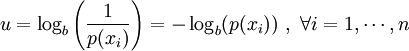
outcomes is defined by

         
   \displaystyle 
   u = \log_b (n)

since the probability of each event is 1 / n, we can write

   \displaystyle 
   u 
   = \log_b \left(\frac{1}{p(x_i)}\right)
   = - \log_b (p(x_i))
   \ , \ \forall i = 1, \cdots , n
 

The average uncertainty \displaystyle \langle u \rangle, with \displaystyle \langle \cdot \rangle being the average operator, is obtained by


   \displaystyle 
   \langle u \rangle
   =
   \sum_{i=1}^{n}
   p(x_i)
   u_i
   =
   -
   \sum_{i=1}^{n}
   p(x_i)
   \log_b (p(x_i))


gray-level histogram -> probability density p(x_k) -> entropy


http://en.wikipedia.org/wiki/Entropy_(information_theory)

Shannon's source coding theorem shows that, in the limit, the average length of the shortest possible representation to encode the messages in a given alphabet is their entropy divided by the logarithm of the number of symbols in the target alphabet.


C.E. Shannon, "A Mathematical Theory of Communication",
Bell System Technical Journal, vol. 27, pp. 379-423, 623-656, July, October, 1948


2.3.4 Visual perception of the image
 
Contrast
http://en.wikipedia.org/wiki/Contrast_(vision
 
Acuity 예민함
http://en.wikipedia.org/wiki/Visual_acuity
 
visual illusions
http://en.wikipedia.org/wiki/Optical_illusion
http://en.wikipedia.org/wiki/Ebbinghaus_illusion
 
 
perceptual grouping -> image segmentation
 
Gestalt theory
http://en.wikipedia.org/wiki/Gestalt_psychology
 
Patterns take precedence over elements and have properties that are not inherent in the elements themselves.
 
 
28p 
 

2.3.5 Image quality
Azriel Rosenfeld, Avinash C. Kak, Digital Picture Processing, Academic Press, 1982

parameter optimization
correlation between images
resolution of small or proximate objects in the image
measures of image similarity (retrieval from image databases)


2.3.6 Noise in image

white noise
http://en.wikipedia.org/wiki/White_noise

-> Gaussian noise

additive noise
http://en.wikipedia.org/wiki/Additive_white_Gaussian_noise

multiplicative noise

quantization noise
http://en.wikipedia.org/wiki/Quantization_noise

impulse noise

-> salt-and-pepper noise
http://en.wikipedia.org/wiki/Salt_and_pepper_noise


unknown about noise properties -> local pre-processing methods
known noise parameters -> image restoration techniques


SNR = signal-to-noise ration
http://en.wikipedia.org/wiki/Signal-to-noise_ratio


2.4 Color images

2.4.1 Physics of color
2.4.2 Color perceived by humans
2.4.3 Color spaces
2.4.4 Palette images
2.4.5 Color constancy

2.5 Cameras: an overview

2.5.1 Photosensitive sensors
2.5.2 A monochromatic camera
2.5.3 A color camera

2.6 Summary
 

'@GSMC > 박래홍: Computer Vision' 카테고리의 다른 글

Ch.10 Image Understanding  (0) 2008.12.15
Ch.9 Object Recognition  (0) 2008.11.25
2.4 Color images & 2.5 Cameras  (0) 2008.10.16
Ch. 6 Segmentation I  (0) 2008.09.20
Ch.1 Introduction  (0) 2008.09.04
posted by maetel